Random Variables III: Continuous Distributions & CLT
Megan Ayers
Math 141 | Spring 2026
Friday, Week 10
Density Curve
Suppose \(X\) is a random variable representing the time (in seconds) it takes for a particle to experience radioactive decay, where \[ f(x) = e^{-x} \qquad \textrm{for } x\geq 0 \]
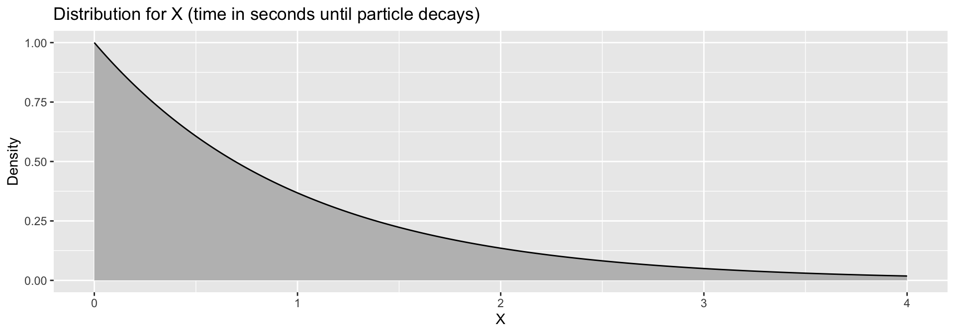
- The probability that it takes between \(1\) and \(2\) seconds to decay is the area under the curve between \(1\) and \(2\). \(P(1 < T < 2) =\)
Density Curve
Suppose \(X\) is a random variable representing the time (in seconds) it takes for a particle to experience radioactive decay, where \[ f(x) = e^{-x} \qquad \textrm{for } x\geq 0 \]
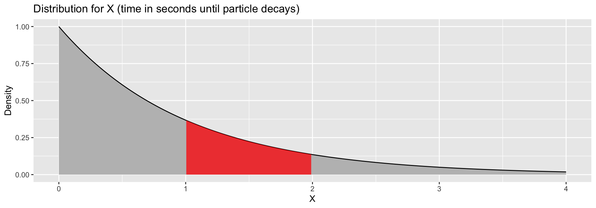
- The probability that it takes between \(1\) and \(2\) seconds to decay is the area under the curve between \(1\) and \(2\). \(P(1 < T < 2) = \color{red}{0.232}\)
Practice with Continuous Random Variables
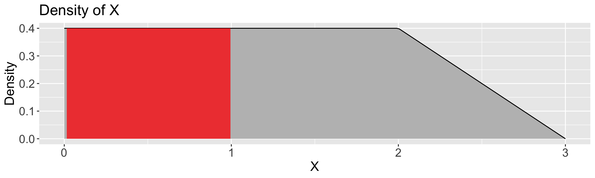
Let \(X\) be a continuous random variable with the density function,
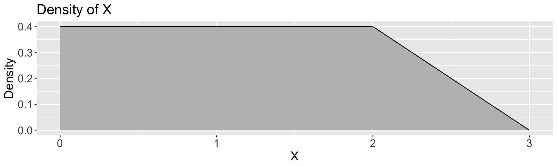
Calculate:
\(P(X \leq 1)\)
\(P(X \leq 2)\)
\(P(2 \leq X \leq 3)\)
Practice with Continuous Random Variables
Let \(X\) be a continuous random variable with the density function,
Calculate:
\(P(X \leq 1) = 1 * 0.4 = \boxed{0.4}\)
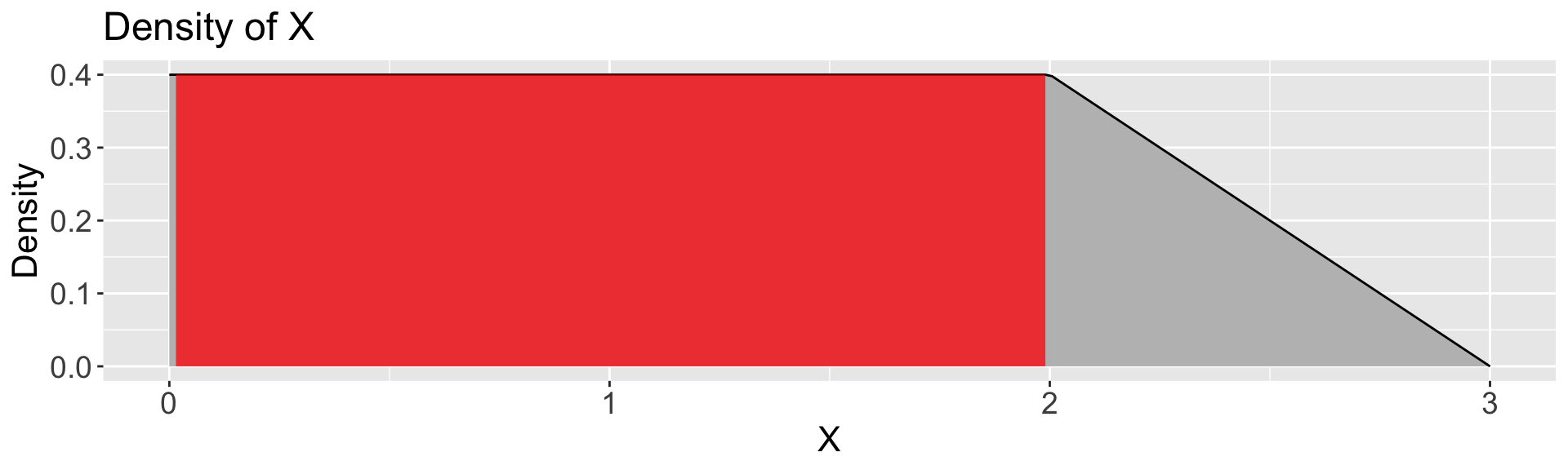
\(P(X \leq 2)\)
\(P(2 \leq X \leq 3)\)
Practice with Continuous Random Variables
Let \(X\) be a continuous random variable with the density function,
Calculate:
\(P(X \leq 1) = 1 * 0.4 = \boxed{0.4}\)
\(P(X \leq 2) = 2 * 0.4 = \boxed{0.8}\)
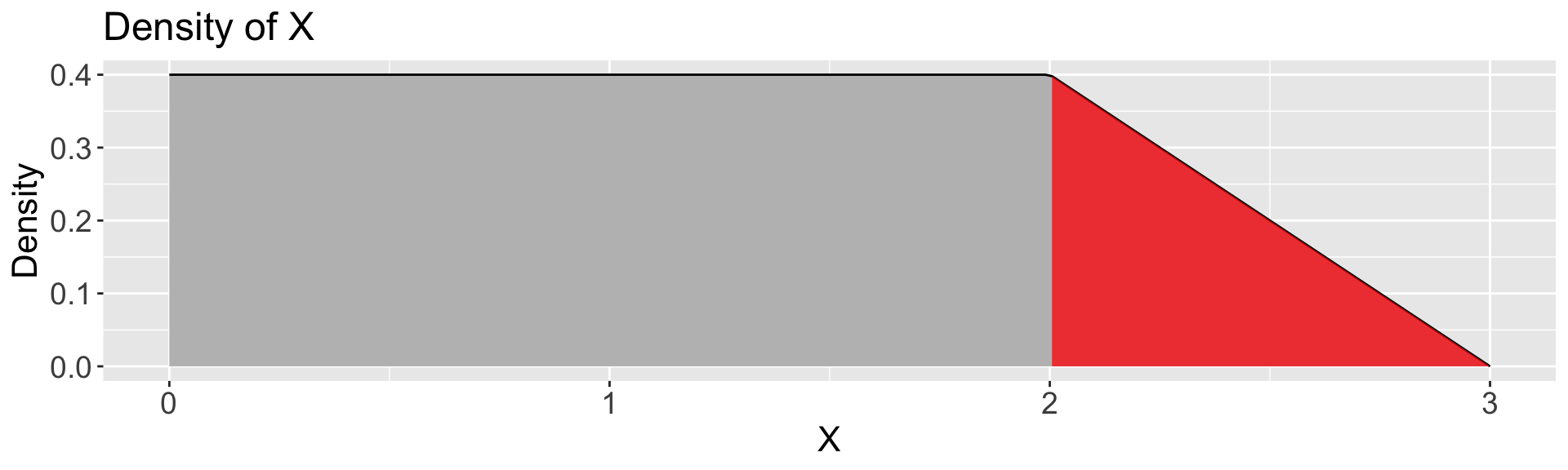
\(P(2 \leq X \leq 3)\)
Practice with Continuous Random Variables
Let \(X\) be a continuous random variable with the density function,
Calculate:
\(P(X \leq 1) = 1 * 0.4 = \boxed{0.4}\)
\(P(X \leq 2) = 2 * 0.4 = \boxed{0.8}\)
\(P(2 \leq X \leq 3) = \frac{1}{2} * 1 * 0.4 = \boxed{0.2}\)
The Normal Distribution
The Normal distribution is defined by two parameters:
- Mean, \(\mu\)
- Standard deviation, \(\sigma\)
Suppose \(X\) follows a Normal(\(\mu\),\(\sigma\)) distribution. The density function is
\[f(x) = \frac{1}{\sqrt{2 \pi \sigma^2}} \cdot\exp \left(\frac{-(x-\mu)^2}{2\sigma^2}\right)\]
(Don’t memorize this!)
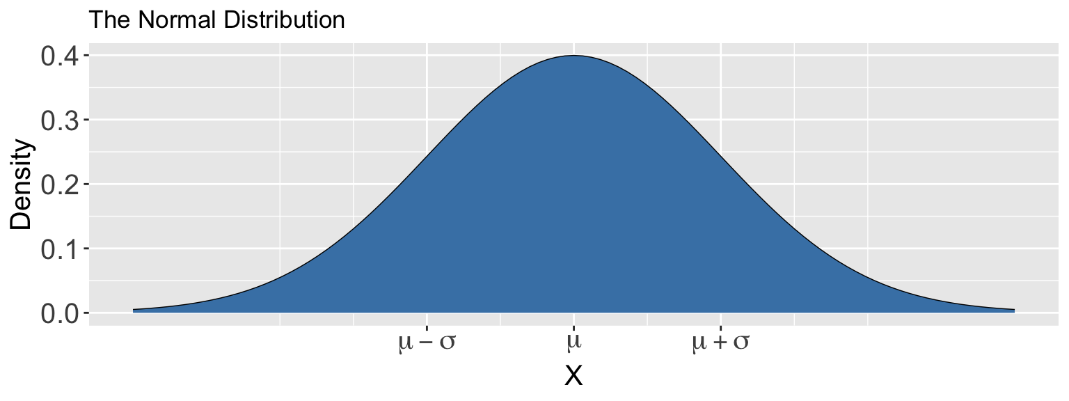
This is the official name for “bell curves”!
Calculating Probabilities
R has built-in functions for calculating probabilities from a normal distribution.
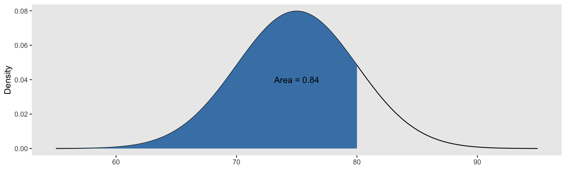
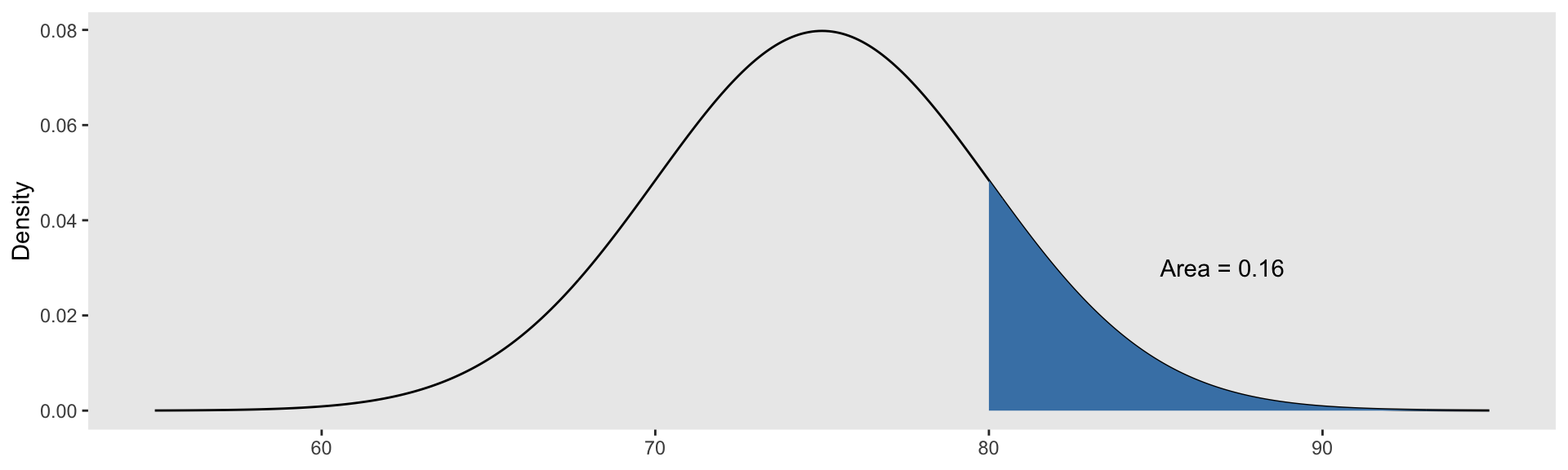
Suppose \(X\sim \text{Normal}(\mu=75, \sigma=5)\). Then:
Calculating Probabilities
R has built-in functions for calculating probabilities from a normal distribution.
Suppose \(X\sim \text{Normal}(\mu=75, \sigma=5)\). Then:
- \(P(X \geq 80) = P(X>80)=\)
Calculating Probabilities
R has built-in functions for calculating probabilities from a normal distribution.
Suppose \(X\sim \text{Normal}(\mu=75, \sigma=5)\). Then:
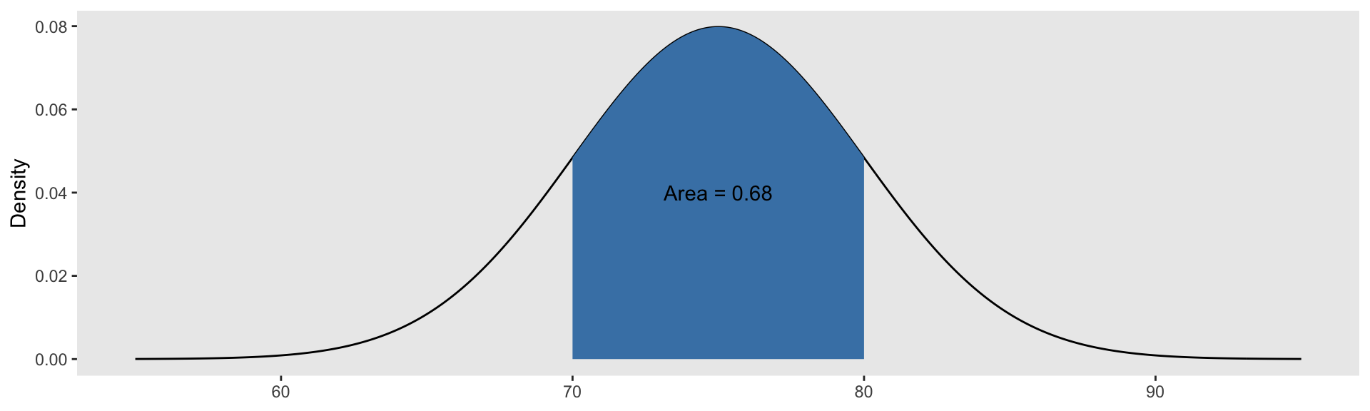
- \(P(70 \leq X \leq 80) = P(X\leq 80) - P(X\leq 70) =\)
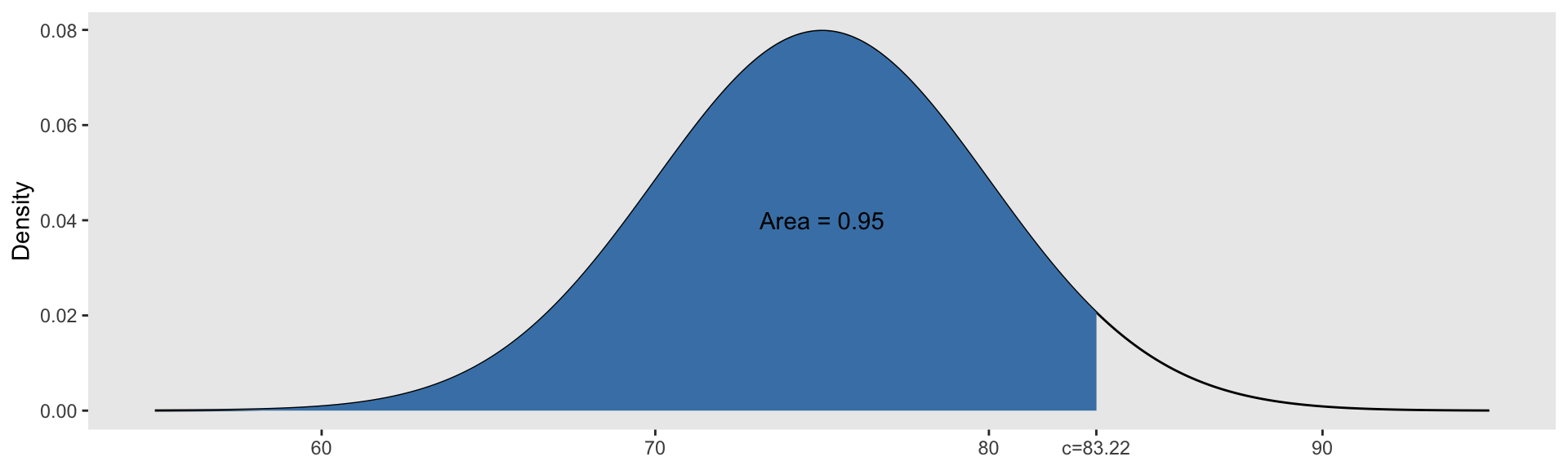
Finding Quantiles
We can also use R to find quantiles of a Normal distribution.
Suppose \(X\sim \text{Normal}(\mu=75, \sigma=5)\). Then:
Scale and Translation Invariance
Suppose \(X\sim\text{Normal}(\mu=0,\sigma=1)\) and \(Y\sim\text{Normal}(\mu=2,\sigma=0.25)\).
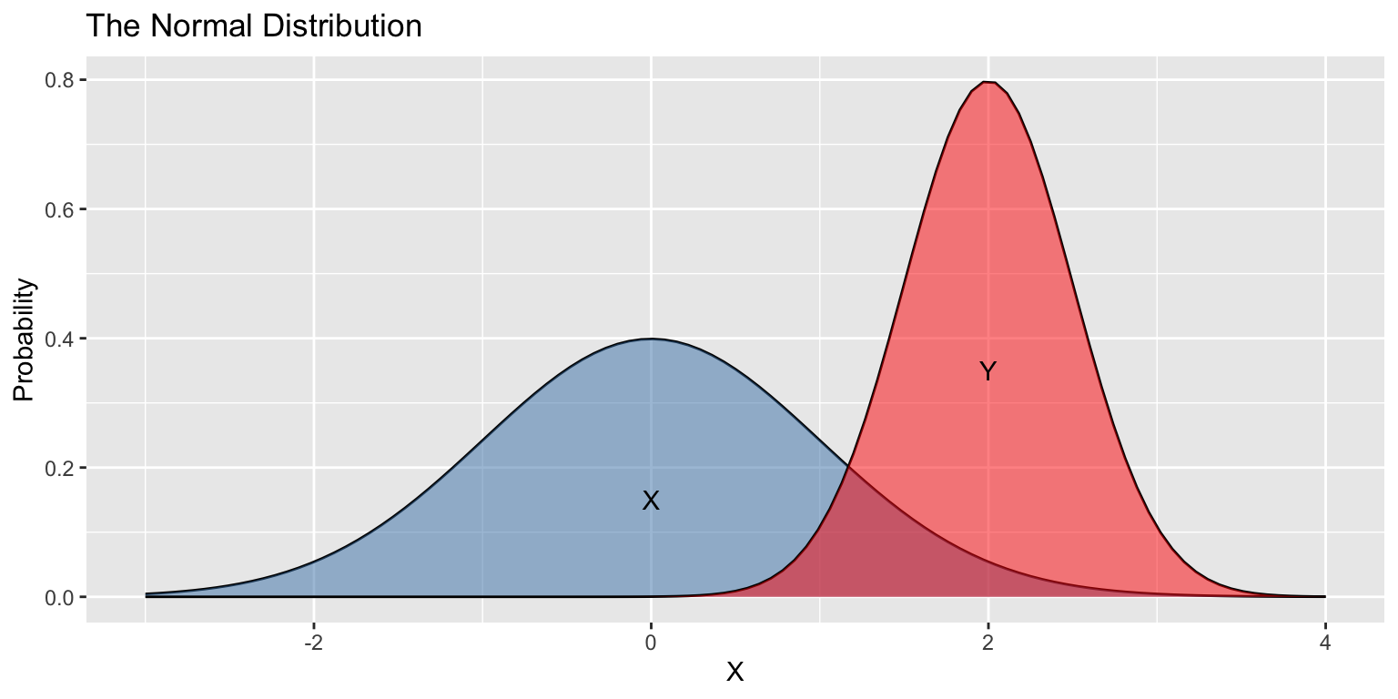
\(X\) and \(Y\) have different means, heights, and widths…
- But the same shapes!
Scale and Translation Invariance
Suppose \(X\sim\text{Normal}(\mu=0,\sigma=1)\) and \(Y\sim\text{Normal}(\mu=2,\sigma=0.25)\).
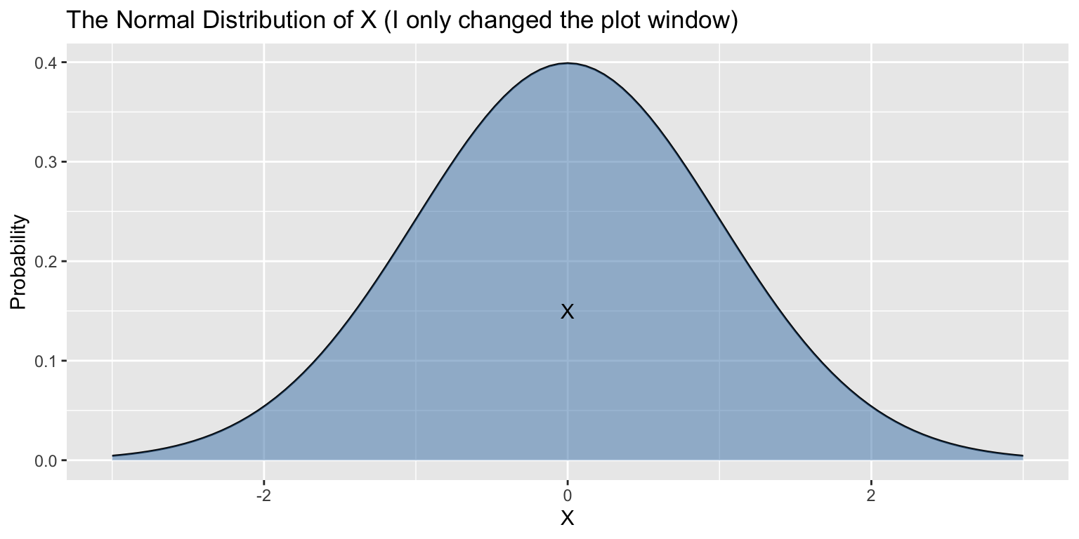
\(X\) and \(Y\) have different means, heights, and widths…
- But the same shapes!
Scale and Translation Invariance
Suppose \(X\sim\text{Normal}(\mu=0,\sigma=1)\) and \(Y\sim\text{Normal}(\mu=2,\sigma=0.25)\).
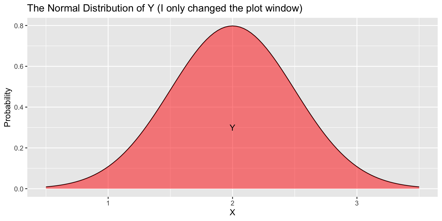
\(X\) and \(Y\) have different means, heights, and widths…
- But the same shapes!
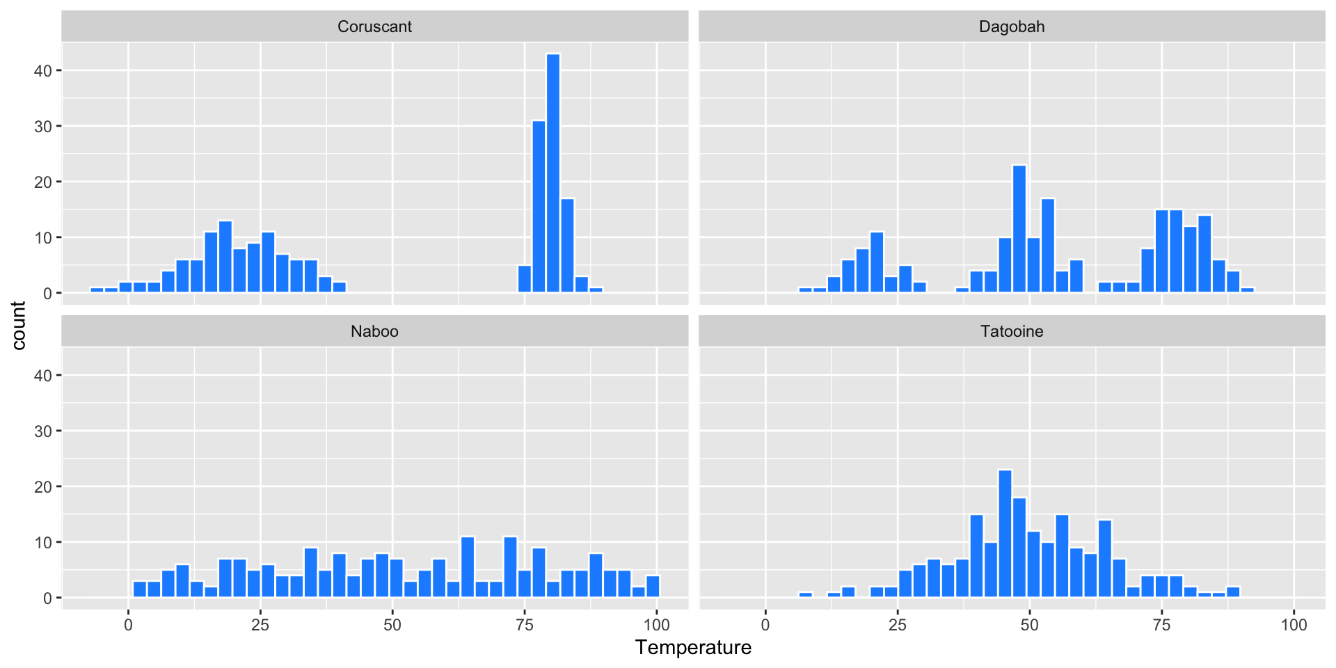
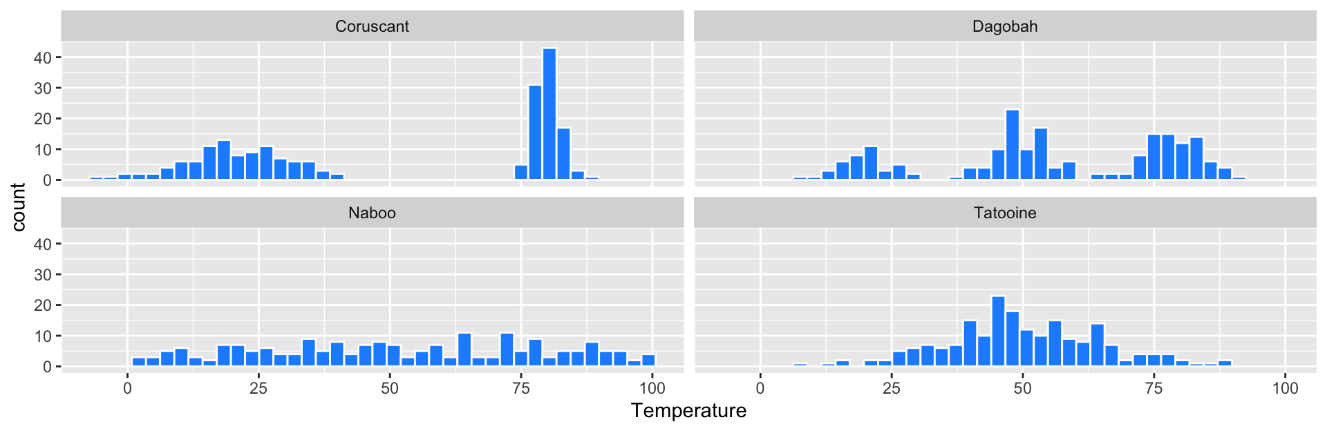
Daily Temperatures
Suppose we’re astronomers studying four far away planets: Naboo, Tatooine, Coruscant, and Dagobah. We have the daily temperature on each of these planets over 200 days:
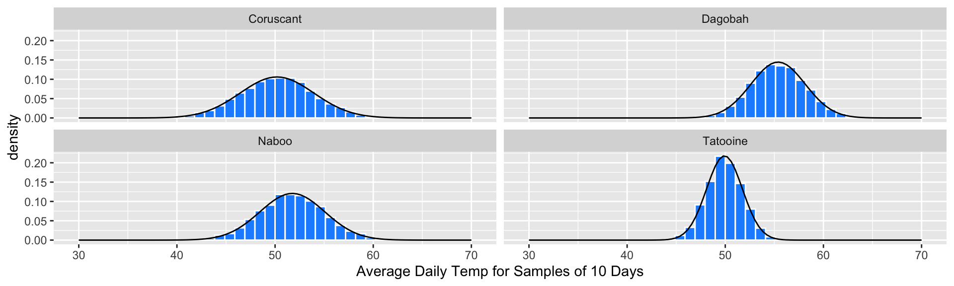
Random Sample Means (n=10)
Suppose we repeatedly take samples of 10 days from each planet, and compute the average temperature \(\bar{x}\) for each sample (these are sampling distributions):
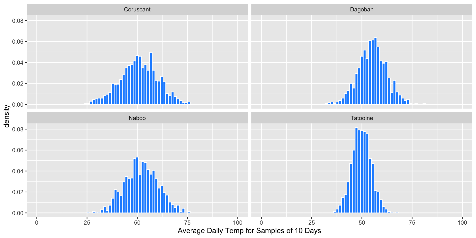
- Q: What does the distribution of sample means look like?
Random Sample Means (n=50)
Suppose we repeatedly take samples of 50 days from each planet, and compute the average temperature \(\bar{x}\) for each sample (these are sampling distributions):
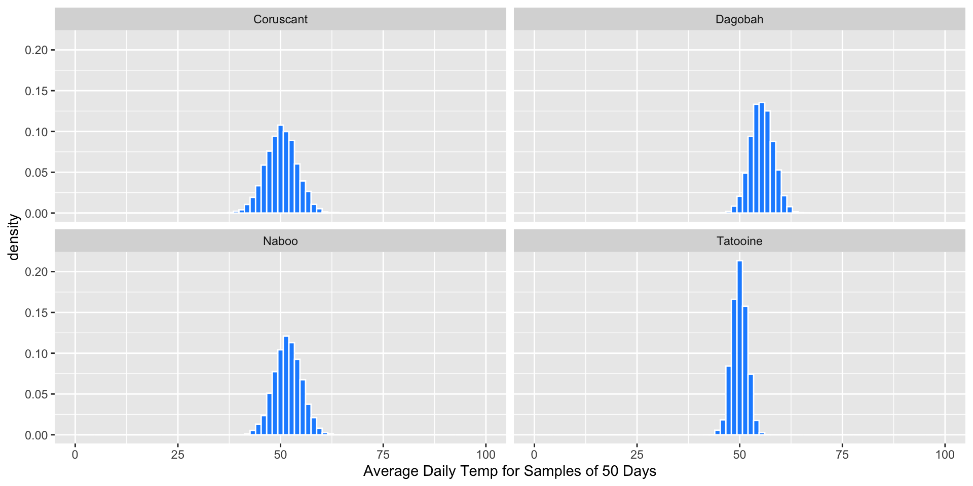
Q: What does the distribution of sample means look like?
Sampling Distributions are Approximately Normal
The sampling distribution for each planet appeared approximately Normal with \(n=50\), regardless of the shape of the population distribution.
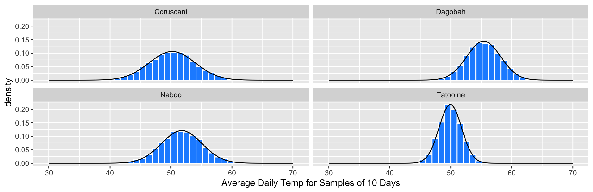
Sampling Distributions are Approximately Normal
The sampling distribution for each planet appeared approximately Normal with \(n=50\), regardless of the shape of the population distribution.
We’ve seen this before! As \(n\) increases,
- Sampling distributions become more Normal
- Variance decreases
- Mean doesn’t change; it is the parameter.