Hypothesis Testing III

Megan Ayers

Math 141 | Spring 2026
Wednesday, Week 8

Goals for today

Discuss decisions in a hypothesis test
- Types of errors
Discuss and learn to compute the power of a hypothesis test

Hypothesis Testing Framework

Have two competing hypotheses:

Null Hypothesis \((H_0)\): “Dull” hypothesis, status quo, random chance, no effect…
Alternative Hypothesis \((H_a)\): The researchers’ conjecture.

Must first take those hypotheses and translate them into statements about the population parameters so that we can test them with sample data.

Example:

\(H_0\): ESP doesn’t exist.

\(H_a\): ESP does exist.

Then translate into a statistical problem!

Q: Using formal statistical/mathematical notation, how should we define these?

\(p\) =

\(H_0\):

\(H_a\):

New Example: Swimming with Dolphins

In 2005, researchers Antonioli and Reveley posed the question “Does swimming with the dolphins help depression?” They recruited 30 US subjects diagnosed with mild to moderate depression. Participants were randomly assigned to either the treatment group (swimming with dolphins) or the control group (swimming without dolphins). After two weeks, each subject was categorized as “showed substantial improvement” or “did not show substantial improvement”.

Here’s a contingency table of improve and group.

dolphins %>%
  count(group, improve)

      group improve  n
1   Control      no 12
2   Control     yes  3
3 Treatment      no  5
4 Treatment     yes 10

\(H_0\):

\(H_a\):

Snapshot of the data:

      group improve
1   Control     yes
2 Treatment      no
3   Control      no
4 Treatment     yes
5   Control      no
6   Control      no
7 Treatment     yes
8   Control      no

Q: How might we generate the null distribution for this scenario?

Penguins Example

Let’s return to the penguins data and ask if flipper length varies, on average, by the sex of the penguin.

Research Question: Does flipper length differ by sex?

Response Variable:

Explanatory Variable:

Statistical Hypotheses:

Exploratory Data Analysis

library(palmerpenguins)

penguins <- palmerpenguins::penguins

penguins %>%
  drop_na(sex) %>%
ggplot(mapping = aes(x = sex,
                     y = flipper_length_mm)) +
  geom_boxplot()

Two-Sided Hypothesis Test

Compute observed test statistic:

penguins %>% drop_na(sex) %>%
  group_by(sex) %>%
  summarize(avg_length = mean(flipper_length_mm))

# A tibble: 2 × 2
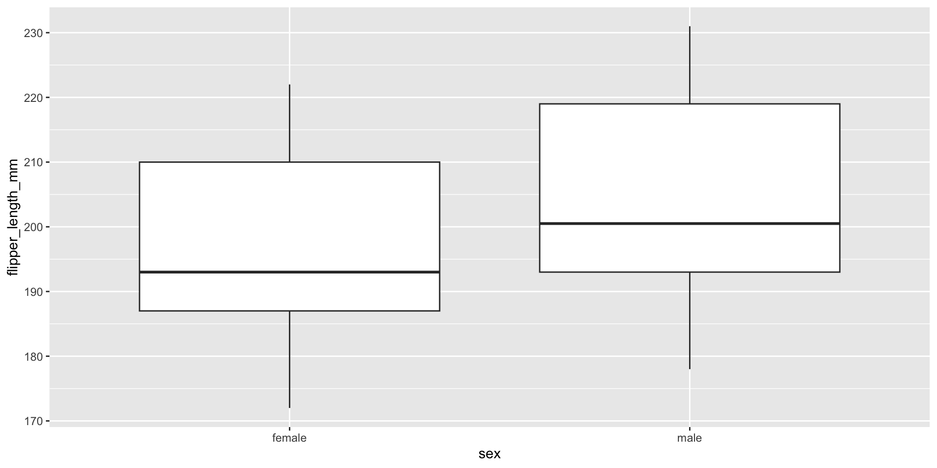
  sex    avg_length
  <fct>       <dbl>
1 female       197.
2 male         205.

\(\rightarrow\) Our test statistic is: 7.1424

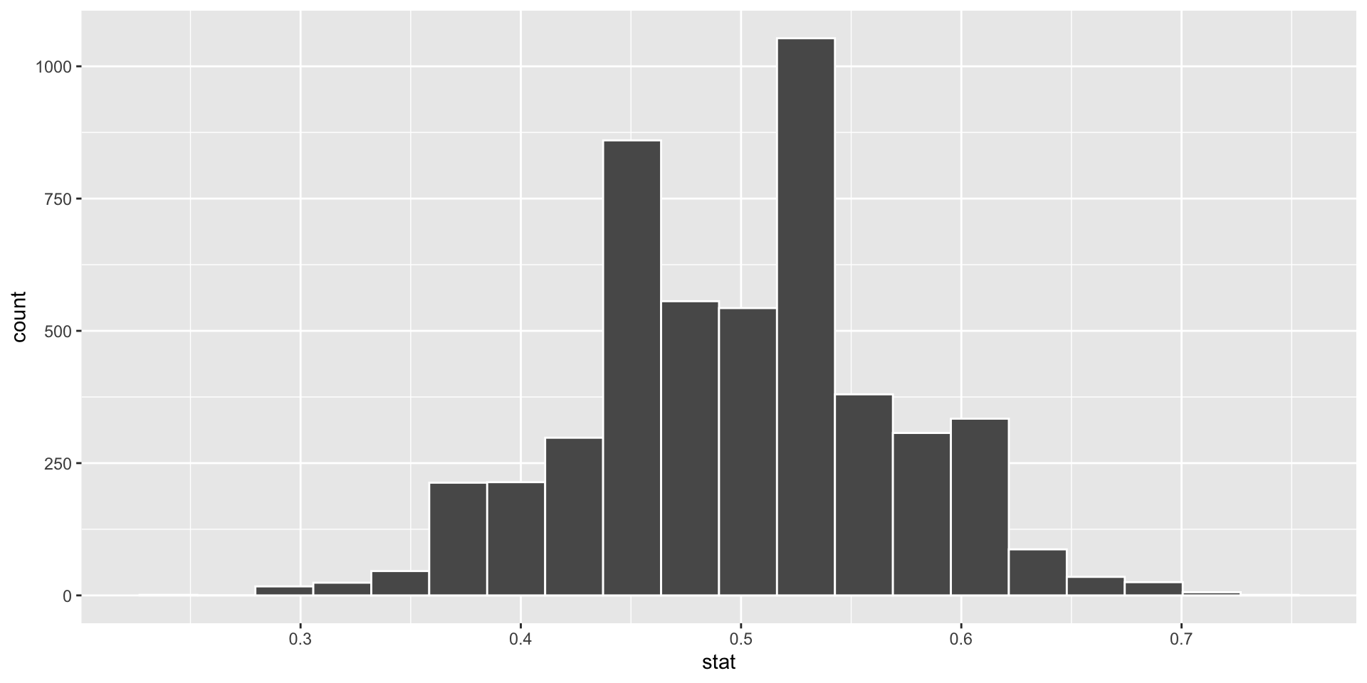
Generate the null distribution by simulating many data sets where gender is shuffled (code not shown for brevity), and visualize null sampling distribution compared to our test statistic:

ggplot(peng_null_stats, aes(x = stat)) +
  geom_histogram(color = "white") +
  geom_vline(xintercept = abs(test_stat),
             color = "deeppink", size = 2) +
  geom_vline(xintercept = -abs(test_stat),
             color = "deeppink", size = 2)

Q: Guesses for p-value?

Two-Sided Hypothesis Test

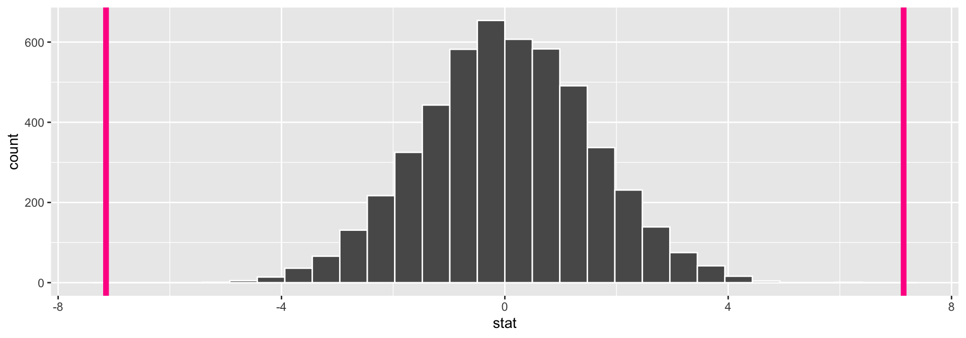
Calculate the p-value for a two-sided test:

# Compute p-value
(p_val <- mean(peng_null_stats$stat > abs(test_stat)) +
   mean(peng_null_stats$stat < -abs(test_stat)))

[1] 0

Interpretation of \(p\)-value: If the mean flipper length does not differ by sex in the population, the probability of observing a difference in the sample means of at least 7.14 mm (in magnitude) is equal to 0.
Conclusion: These data represent evidence that flipper length does vary by sex.

Now: A closer look at the conclusions of a hypothesis test

Hypothesis Testing: Decisions, Decisions

Once you get to the end of a hypothesis test you make one of two decisions:

P-value is small.
- I have evidence for \(H_a\). Reject \(H_0\).
P-value is not small.
- I don’t have evidence for \(H_a\). Fail to reject \(H_0\).

Sometimes we make the correct decision. Sometimes we make a mistake.

Hypothesis Testing: Decisions, Decisions

Let’s create a table of potential outcomes on the board.

\(\alpha\) = prob of Type I error under repeated sampling = prob reject \(H_0\) when it is true

\(\beta\) = prob of Type II error under repeated sampling = prob fail to reject \(H_0\) when \(H_a\) is true.

Hypothesis Testing: Decisions, Decisions

We should set \(\alpha\) level beforehand.

Use \(\alpha\) to determine “small” for a p-value.

P-value is ~~small~~ \(< \alpha\).
- \(\rightarrow\) I have evidence for \(H_a\). Reject \(H_0\).
P-value is ~~not~~ ~~small~~ \(\geq \alpha\).
- \(\rightarrow\) I don’t have evidence for \(H_a\). Fail to reject \(H_0\).

Hypothesis Testing: Decisions, Decisions

Open Question: How do I select \(\alpha\)?

Will depend on the convention in your field (0.05 is common).
Want a small \(\alpha\) and a small \(\beta\). But they are related.
- The smaller \(\alpha\) is the larger \(\beta\) will be.
Choose a lower \(\alpha\) (e.g., 0.01, 0.001) when the Type I error is worse and a higher \(\alpha\) (e.g., 0.1) when the Type II error is worse.

Q: What are some examples of when Type I errors are worse than Type II errors? Examples when the opposite is true?

Hypothesis Testing: Decisions, Decisions

Open Question: How do I select \(\alpha\)?

Will depend on the convention in your field (0.05 is common).
Want a small \(\alpha\) and a small \(\beta\). But they are related.
- The smaller \(\alpha\) is the larger \(\beta\) will be.

Q: Can’t easily compute \(\beta\) (probability of failing to reject a false null hypothesis). Why?
Important related concept:
- Power = probability reject \(H_0\) when the alternative is true.

Q: Why is power important when designing an experiment?

Example

Suppose we want to test whether someone can detect AI-generated text from real text. We show a participant 10 short passages that are each either written by a human or an AI agent, and ask them to identify which are written by AI. Suppose the participant’s true (long-run) detection rate is 70%.

\(H_0\):

\(H_a\):

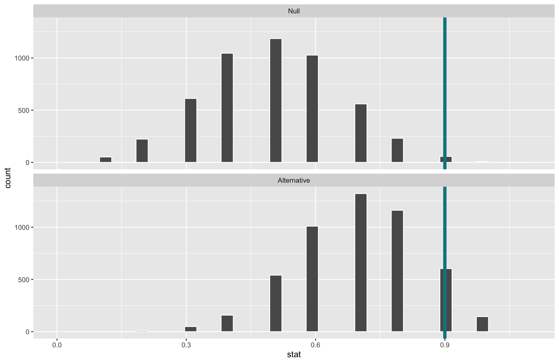
When \(\alpha=0.05\), they need 9 or more correct for a small enough p-value to reject \(H_o\).
When \(\alpha=0.05\), the power of this test is 0.15.

Why is the power so low? Our power is very much not “unlimited” :(

What aspects of the test could we change to increase the power of the test?

Example

Suppose we want to test whether someone can detect AI-generated text from real text. We show a participant 10 50 short passages that are each either written by a human or an AI agent, and ask them to identify which are written by AI. Suppose the participant’s true (long-run) detection rate is 70%.

What will happen to the power of the test if we increase the sample size?

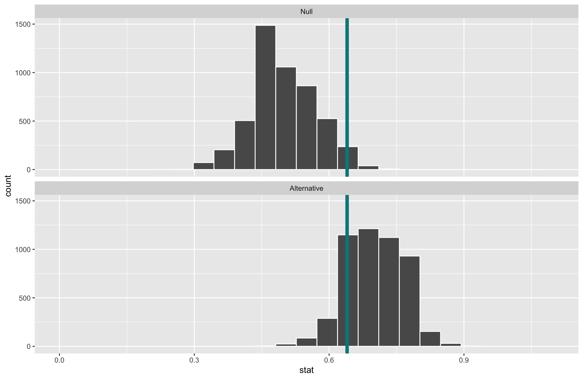
Increasing the sample size narrows the sampling distributions and increases the power.
When \(\alpha\) is set to \(0.05\) and the sample size is now 50, the power of this test is 0.87.

Example

What will happen to the power of the test if we increase \(\alpha\) to 0.1?

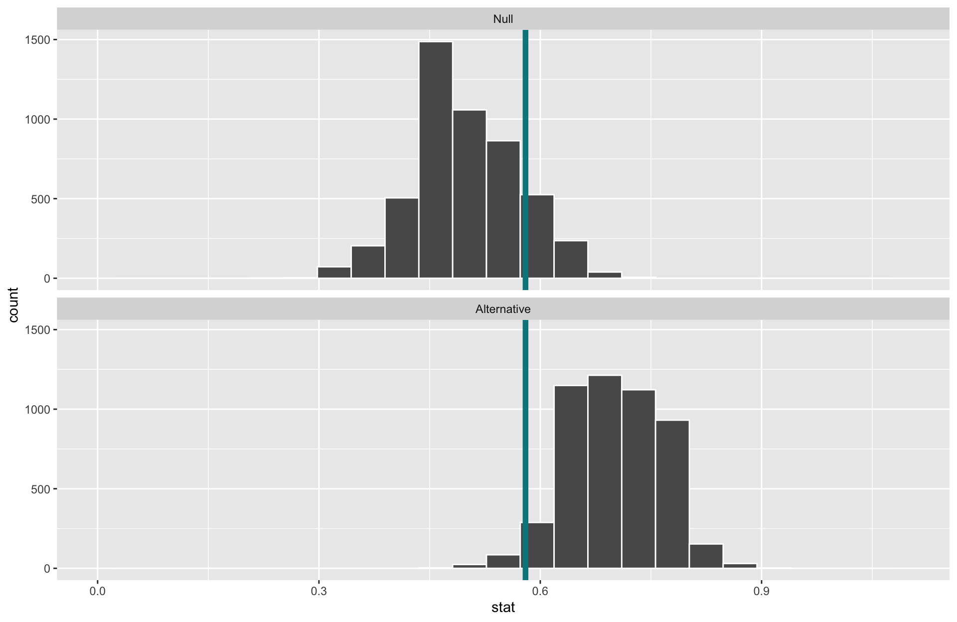
Increasing \(\alpha\) increases the power.
- Decreases \(\beta\).
- (But remember, also increasing our chances of false alarms)
When \(\alpha\) is set to \(0.1\) and the sample size is 50, the power of this test is 0.98!

Example

What will happen to the power of the test if the participant is even better at detecting AI?

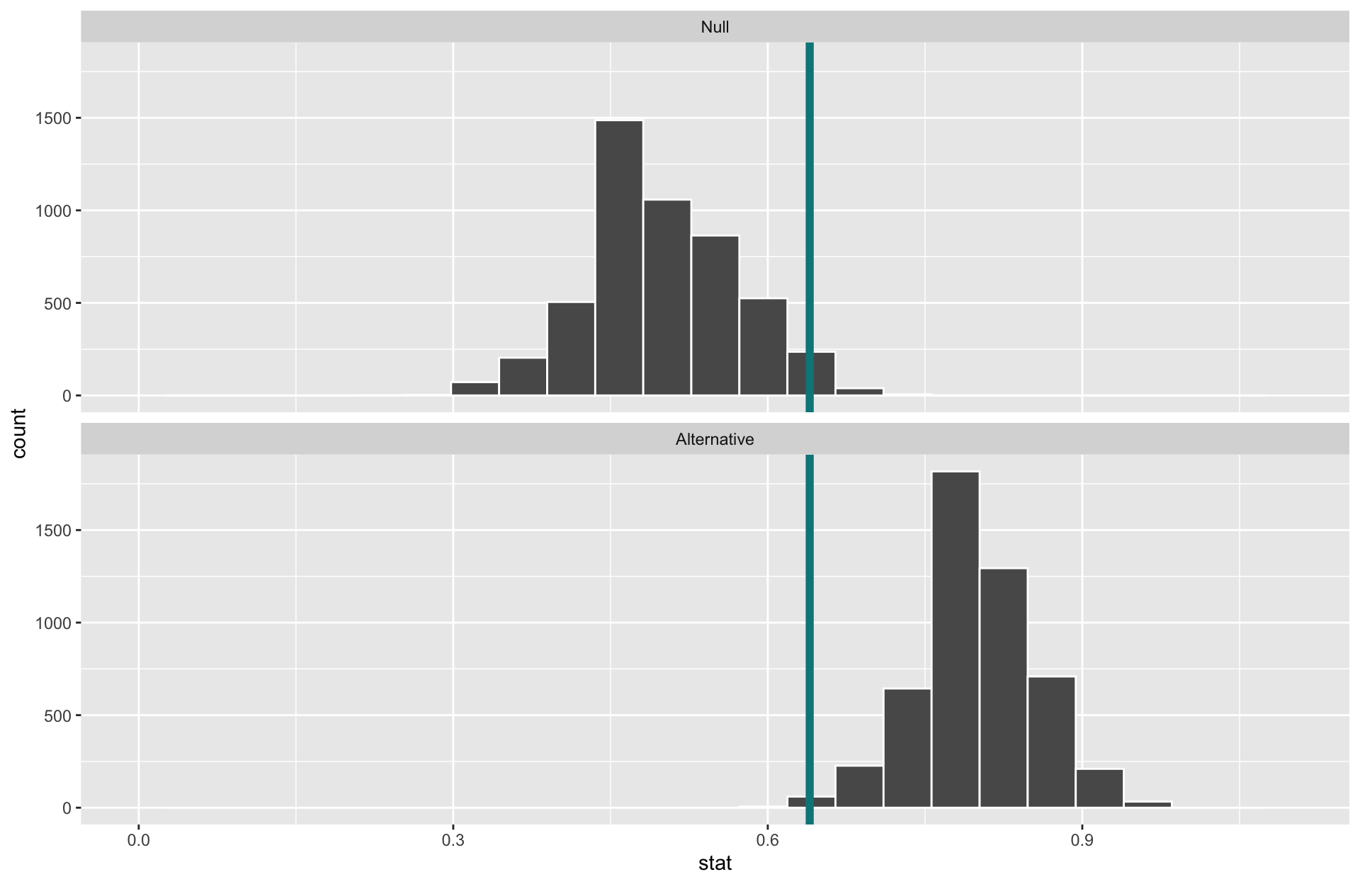
Effect size: Difference between true value of the parameter and null value.
- Often standardized.
Increasing the effect size increases the power.
When \(\alpha\) is set back to \(0.05\), the sample size is 50, and the true probability of detecting AI is 0.8, the power of this test is 0.998.

Computing Power

Generate a null distribution:

# Generate null distribution
null_stats <- data.frame(correct = c(0, 1)) %>% 
  rep_sample_n(size = 50, replace = TRUE,
               reps = 5000) %>%
  group_by(replicate) %>%
  summarize(stat = mean(correct))

ggplot(data = null_stats, mapping = aes(x = stat)) +
  geom_histogram(bins = 20, color = "white")

Computing Power

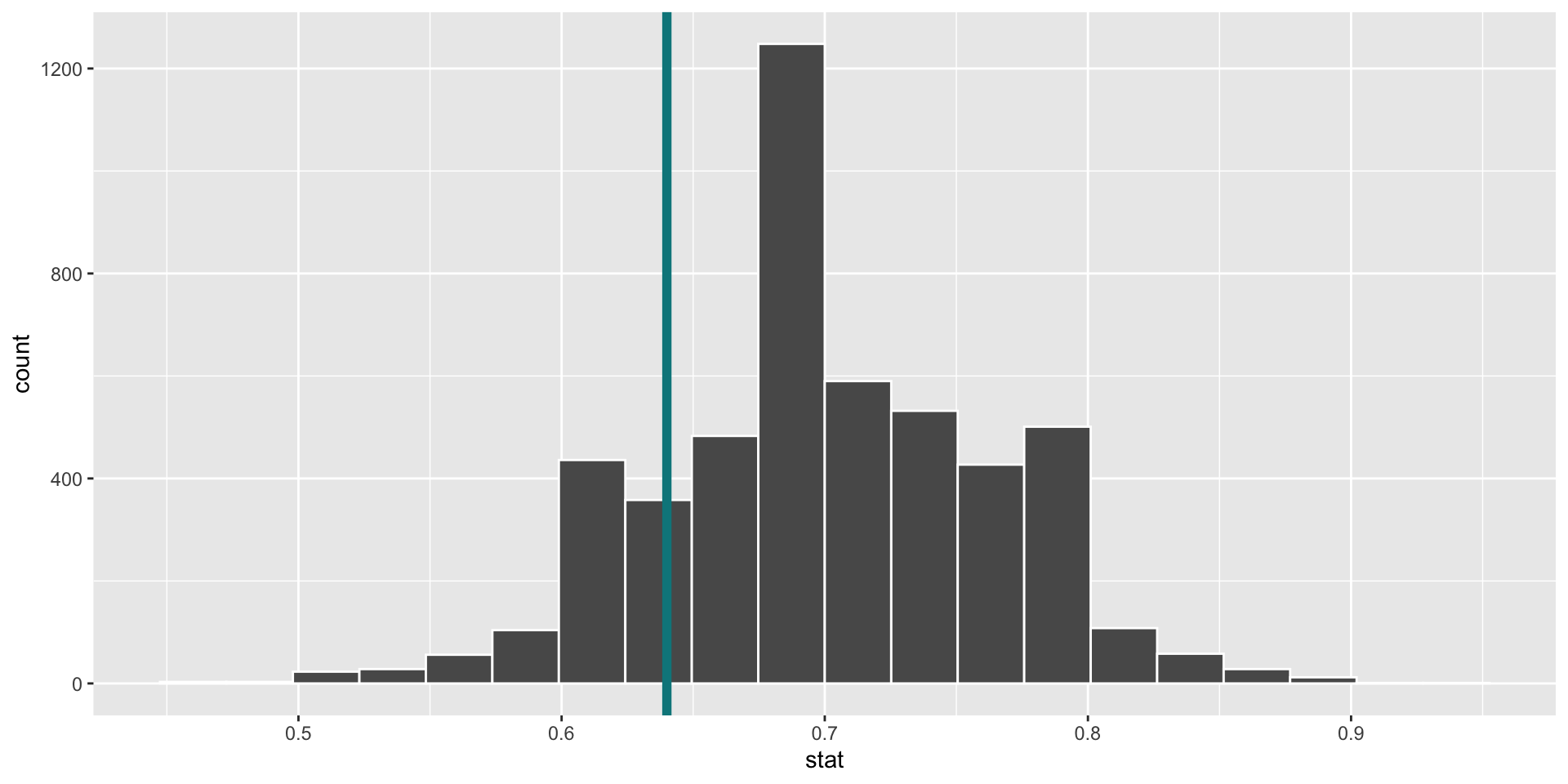
Determine the “critical value(s)” where \(\alpha = 0.05\) (careful with discrete distributions).

quantile(null_stats$stat, 0.95)

 95% 
0.62

mean(null_stats$stat >= 0.62)  # 31/50

[1] 0.0518

mean(null_stats$stat >= 0.64)  # 32/50

[1] 0.0246

ggplot(data = null_stats, mapping = aes(x = stat)) +
  geom_histogram(bins = 20, color = "white") +
  geom_vline(xintercept = 0.64, size = 2,
             color = "turquoise4")

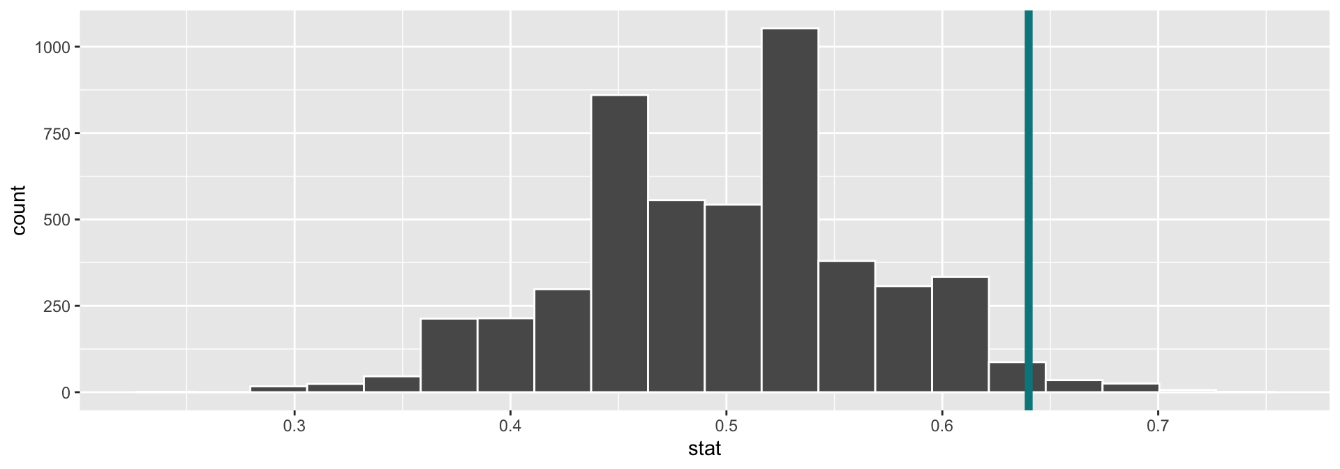
Computing Power

Construct the alternative distribution. This usually requires a leap of faith - we need to assume a parameter under the alternative hypothesis!
- Draw on any existing evidence (ex. a pilot study) to justify your assumption

alt_stats <- data.frame(correct = rep(c(0, 1),
                        times = c(3, 7))) %>% 
  rep_sample_n(size = 50, replace = TRUE,
               reps = 5000) %>%
  group_by(replicate) %>%
  summarize(stat = mean(correct))

ggplot(data = alt_stats, mapping = aes(x = stat)) +
  geom_histogram(bins = 20, color = "white") +
  geom_vline(xintercept = 0.64,
             size = 2, color = "turquoise4")

Computing Power

Find the probability of the critical value or more extreme under the alternative distribution.

alt_stats %>%
  summarize(power = mean(stat >= 0.64))

# A tibble: 1 × 1
  power
  <dbl>
1 0.849

Thoughts on Power

Q: We saw how \(\alpha\), \(n\), and the effect size affected power. What aspects of the test do we actually have control over?
Q: Why is it easier to set \(\alpha\) than to set \(\beta\) or power?
Although it can be challenging, considering power before collecting data is very important!
Under-powered studies carry large risks
- Grants often require power analyses to justify funding
- Type II errors can be dangerous depending on the setting

Next time:

\(p\)-value pitfalls