Confidence Intervals II
Megan Ayers
Math 141 | Spring 2026
Wednesday, Week 7
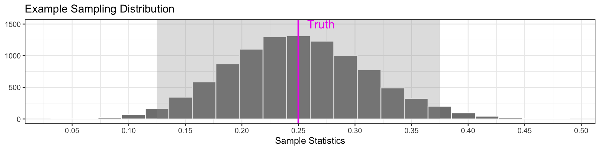
Sampling Distributions can determine the Margin of Error
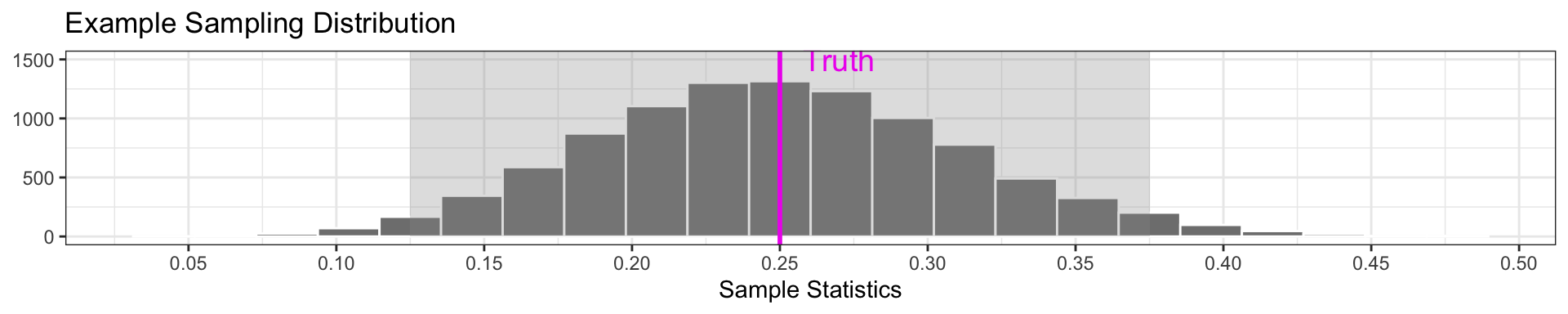
Implication: in the sampling distribution, 95% of sample statistics lie in the range: \[ \text{Parameter} \pm 2*\text{Standard Error} \] where the Standard Error is the standard deviation of the sampling distribution
So, 95% of sample statistics are within \(2*\mathrm{SE}\) from the parameter!
Thus, 95% confidence intervals usually take the form:
\[ \textrm{Statistic }\pm 2*\textrm{Standard Error (SE)} \]
- We typically estimate the SE (i) with the bootstrap, or (ii) with a formula
Example: Reproduction Rate for Covid-19
Researchers are interested in the COVID-19 reproduction rate (the average number of individuals each infected person further infects)
Sample 50 infected individuals and perform contract tracing.
  infected  n
1        0  5
2        1 13
3        2 14
4        3 12
5        4  5
6        6  1
mean_infected
1 2.06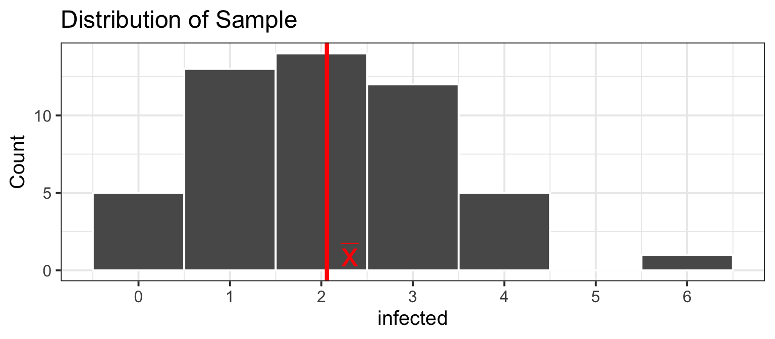
Goal: Create an interval of plausible values for the reproduction rate.
Q: What is the population? What is the parameter?
Q: What is the sample? What is the statistic?
Bootstrap Reproduction Rate
We can use our sample to create a 95% confidence interval. What is each step doing, and why?
- Step 1:
- Step 2:
- Step 3:

- Step 5:
\[ \bar x \pm 2 \cdot SE \implies 2.06 \pm 2 \cdot 0.181 \]
Bootstrap Reproduction Rate
We can use our sample to create a 95% confidence interval.
- Create the bootstrap samples:
- Compute bootstrap statistics within each bootstrap sample:
- Graph the bootstrap distribution to check shape:
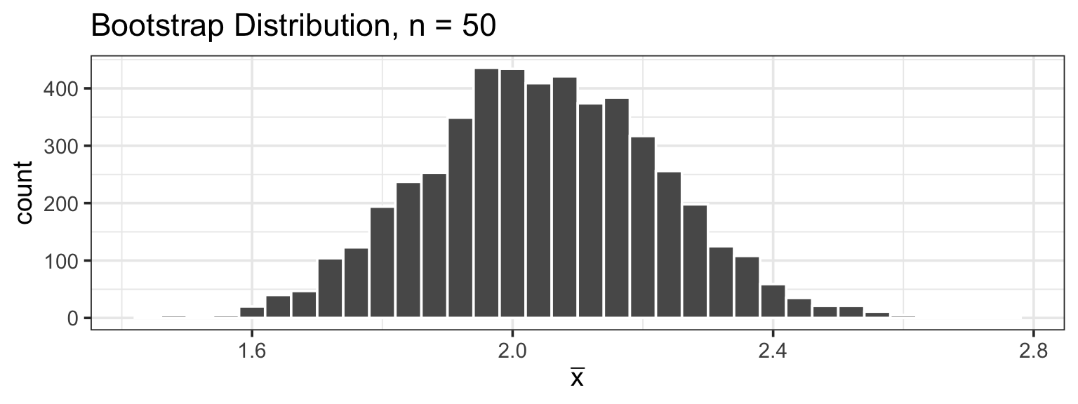
- Estimate the standard error
- Because the bootstrap distribution is bell-shaped, we use \(2 \times\) the estimated SE as our margin of error to create a 95% confidence interval
\[ \bar x \pm 2 \cdot SE \implies 2.06 \pm 2 \cdot 0.181 \]
Review: Percentiles and Quantiles
- For a number \(k\) between \(0\) and \(100\), the \(k\)th percentile of a distribution is the value so that \(k\%\) of the data is less than or equal to that value.
- The median is the 50th percentile of a distribution
- 1st/3rd quartiles (Q1/Q3) are the 25th and 75th percentiles, respectively.
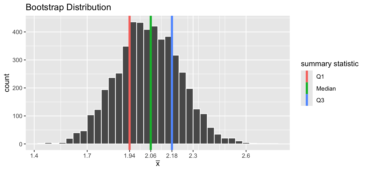
- For a number \(p\) between \(0\) and \(1\), the \(p\) quantile of a distribution is the value so that a proportion \(p\) of the data is less than or equal to that value.
- The median is the \(0.5\) quantile of a distribution
- 1st/3rd quartiles (Q1/Q3) are the \(0.25\) and \(0.75\) quantiles, respectively.
Quantiles and Percentiles
By definition, 2.5% of the data is less than the .025 quantile, and 2.5% of the data is greater than the .975 quantile
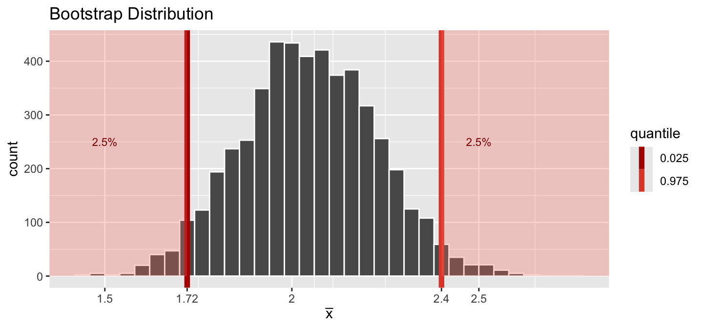
- This means that 95% of the data is between the .025 and the .975 quantiles.
Quantiles and Percentiles
By definition, 2.5% of the data is less than the .025 quantile, and 2.5% of the data is greater than the .975 quantile
- This means that 95% of the data is between the .025 and the .975 quantiles
For sampling distributions that are bell-shaped, the .025 quantile is about \(2\cdot SE\) below the mean, and the .975 quantile is about \(2\cdot SE\) above the mean
So using the .025 and .975 quantiles is roughly equivalent to forming a 95% CI as: \(\text{Statistic} \pm 2*\text{SE}\)!
95% Confidence Interval: 2 ways
- \(\color{red}{\text{Statistic} \pm 2*\text{SE}}\)
- \(\mathrm{Statistic} \ (\bar{x}) = 2.06\)
- \(\mathrm{SE} = 0.18\)
- \(95\% \ \mathrm{CI} = 1.70 \ \text{to} \ 2.42\)
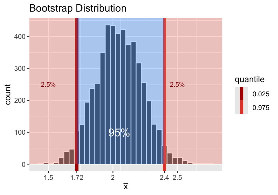
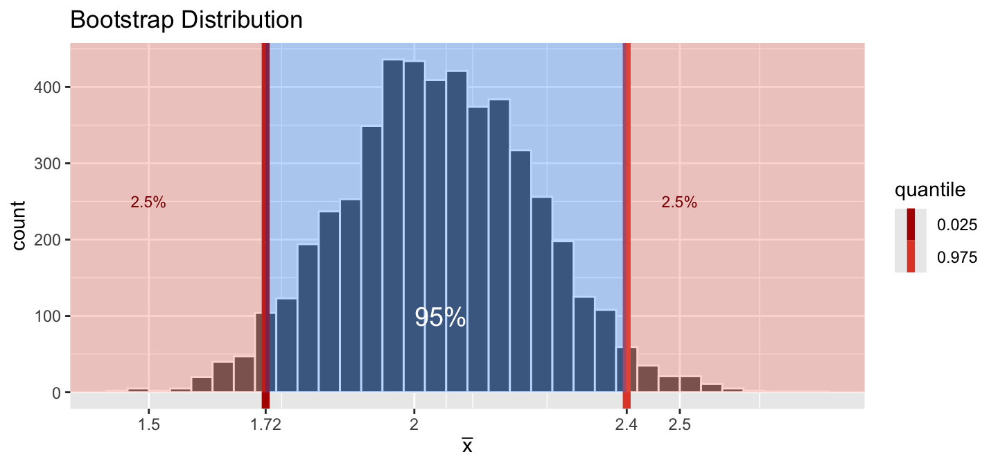
The Percentile Method: Example
- Suppose we want to construct a 90% confidence interval for the reproduction rate
- Find the .05 and .95 quantiles in the bootstrap distribution.
- 90% of bootstrap sample statistics will be between these values
- We can use the
quantilefunction in R to calculate the .05 and .95 quantiles
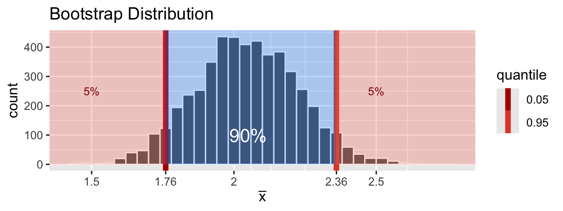
The Percentile Method: Example
- Suppose we want to construct a 90% confidence interval for the reproduction rate
- Find the .05 and .95 quantiles in the bootstrap distribution.
- 90% of bootstrap sample statistics will be between these values

- Our 90% confidence interval is therefore 1.76 to 2.36
Misunderstanding 1
Suppose we wish to estimate the number of hours a Reed student sleeps on a typical night. We obtain the following 95% confidence interval: \((7.86, 8.34)\)
- A 95% confidence interval does not contain 95% of observations in the population.
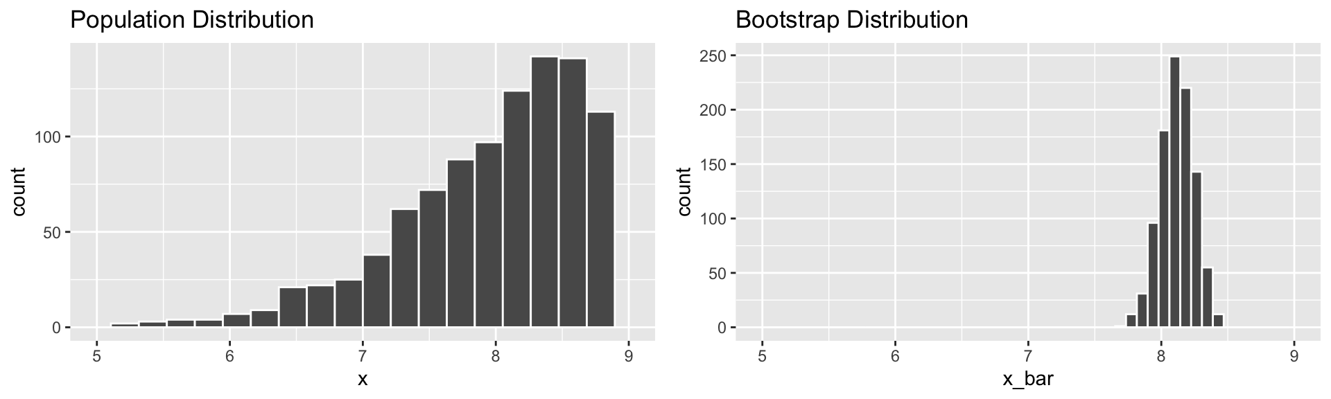
Misunderstanding 1
Suppose we wish to estimate the number of hours a Reed student sleeps on a typical night. We obtain the following 95% confidence interval: \((7.86, 8.34)\)
- A 95% confidence interval does not contain 95% of observations in the population.
- Saying that 95% of all Reed students sleep between 7.86 and 8.34 hours should just feel wrong. That’s a pretty narrow interval!
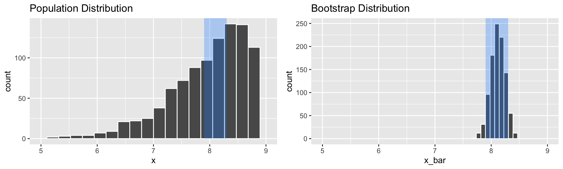
Misunderstanding 2
- A 95% confidence interval does not mean that 95% of all sample means fall within the given range.
Misunderstanding 2
- A 95% confidence interval does not mean that 95% of all sample means fall within the given range.

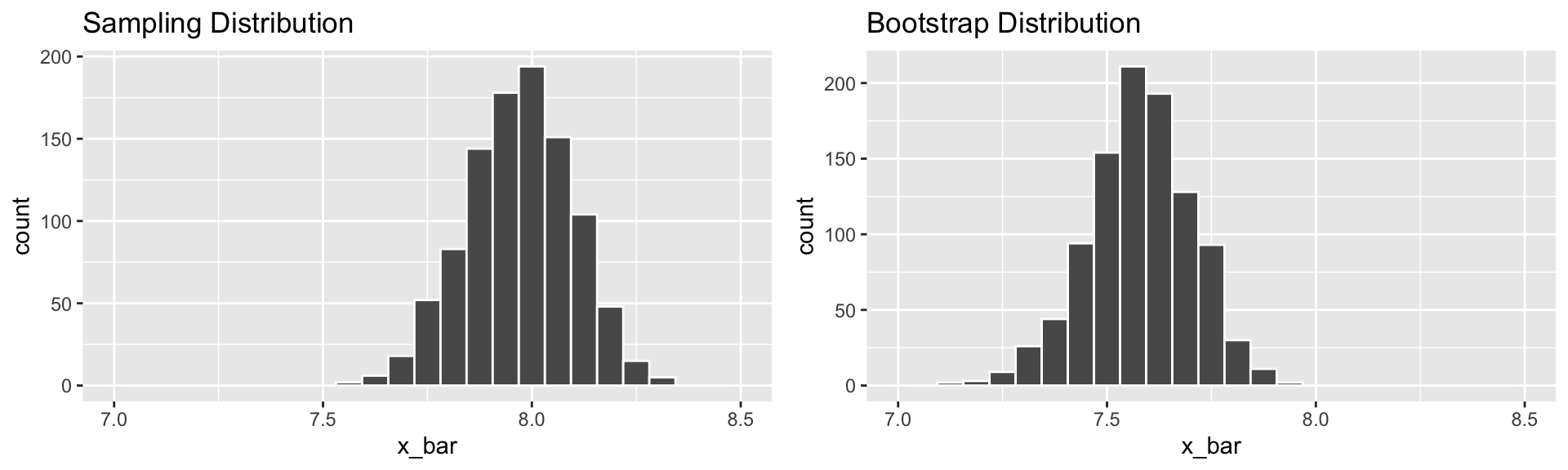
- Q: Why do the sampling distribution and bootstrap distribution look different?
Misunderstanding 2
- A 95% confidence interval does not mean that 95% of all sample means fall within the given range.
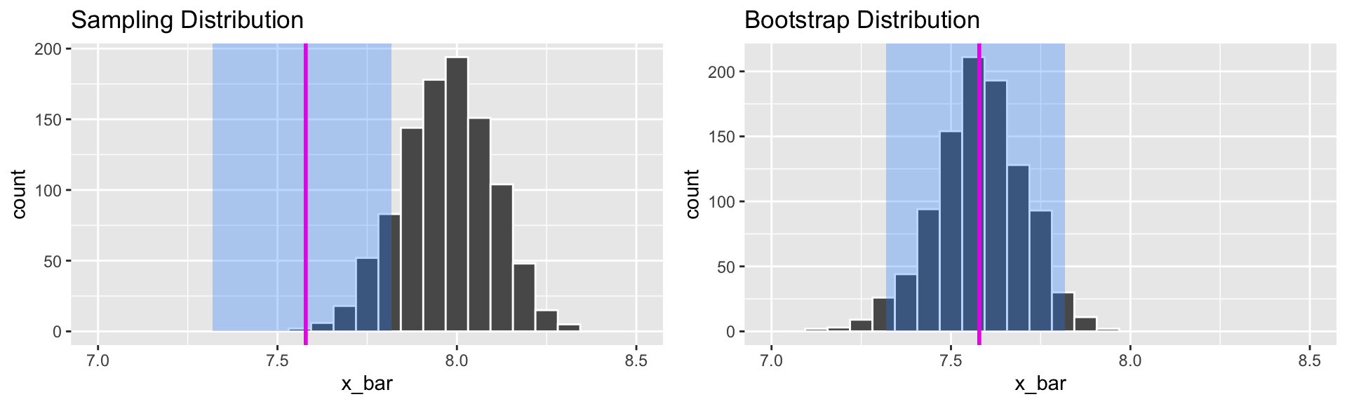
- Q: Why do the sampling distribution and bootstrap distribution look different?