Point Estimates
- To estimate a population parameter, we can use a sample statistic.
- Ex: You’re hosting a pizza party for 200 people, and need to know what proportion \(p\) of vegetarian pizza to order.
- Idea: Ask a (random) sample of attendees about their pizza preference and use the proportion \(\widehat{p}\) in the sample as an estimate for the total proportion \(p\).
- Your sample statistic, \(\widehat{p}\), is a good guess for the population parameter.
- Terminology: We sometimes call our sample statistic a point estimate.
Point Estimates vs. Interval Estimates
- A sample statistic is a good guess for the population parameter, but not the whole story
- Q: After polling pizza party attendees, you find \(\widehat{p} = 0.33\). What factor(s) determine your (un)certainty in this estimate?
- It may be preferable to estimate the proportion using a range of values, with smaller intervals corresponding to precision.
With just \(n = 9\) people, you might give a range of \(0.03\) to \(0.63\) for \(p\).
But with \(n = 48\), you might instead give the range \(0.20\) to \(0.46\).
- We call these ranges interval estimates.
Confidence Interval Estimates
A confidence interval estimate for a parameter usually takes the form \[
\textrm{Statistic }\pm \textrm{ Margin of Error (ME)}
\]
The confidence interval gives a range of plausible values for the parameter.
- e.g., when sampling pizza preferences with \(n=48\), we estimate \(p\) using the interval
\[
0.20 \textrm{ to } 0.46 \qquad \textrm{ or } \qquad \underbrace{0.33}_{\text{Statistic ($\widehat{p}$)}} \pm \ \ \ \underbrace{0.13}_{\text{ME}}
\]
The Margin of Error determines the width of the interval (\(2*\text{Margin of Error}\))
- e.g., in our pizza interval, the width is: \[
0.46 - 0.20 = 0.26 = 2 * \underbrace{0.13}_{\text{ME}}
\]
Q: How should we choose our Margin of Error? (think conceptually)
Confidence Intervals using the Sampling Distribution
Goal: Figure out a reasonable Margin of Error
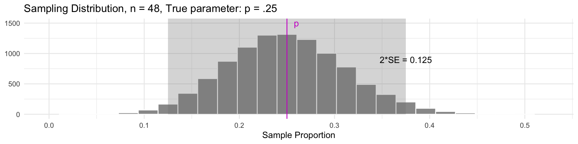
In our example, suppose \(p = 0.25\) (i.e., 25% of all party attendees prefer vegetarian)
For approximately bell-shaped sampling distributions, 95% of all sample statistics are within 2 SE of the parameter.
- This also means that for 95% of all samples, the parameter will be within a distance of 2 SE of the sample statistic (every sample in the gray region)
Confidence Intervals
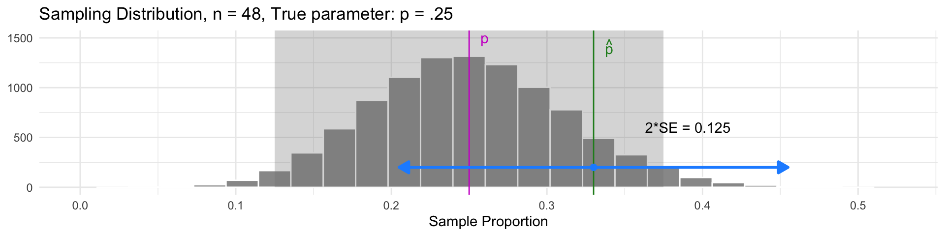
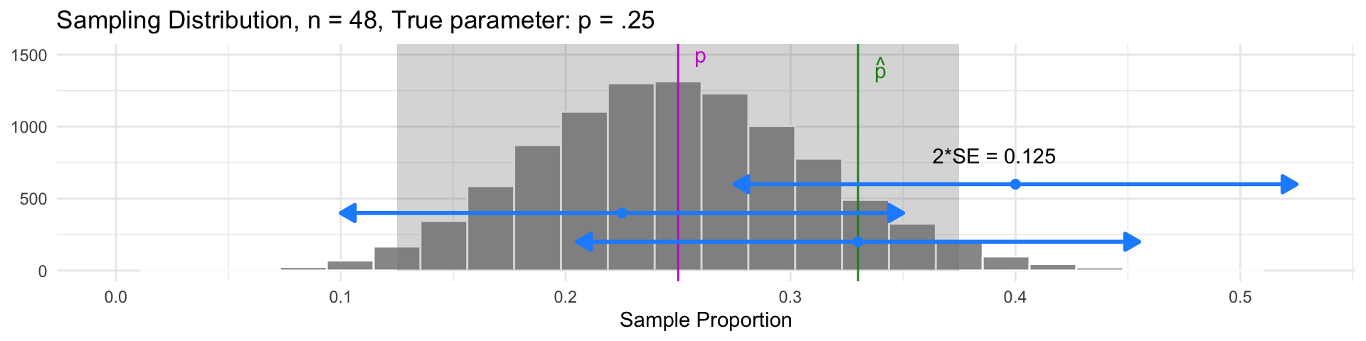
Idea: Build an interval centered at the sample statistic, with a margin of error of \(2\cdot SE\):
\[
\widehat{p} \pm 2\cdot \textrm{SE}
\]
- This interval will contain the parameter \(p\) in 95% of samples!
- The interval for our sample was \(0.33 \pm 0.125\), which does contain the parameter \(p\)
Interval Estimates
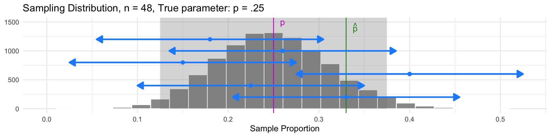
Idea: Build an interval centered at the sample statistic, with a margin of error of \(2\cdot SE\):
\[
\widehat{p} \pm 2\cdot \textrm{SE}
\]
- This interval will contain the parameter \(p\) in 95% of samples!
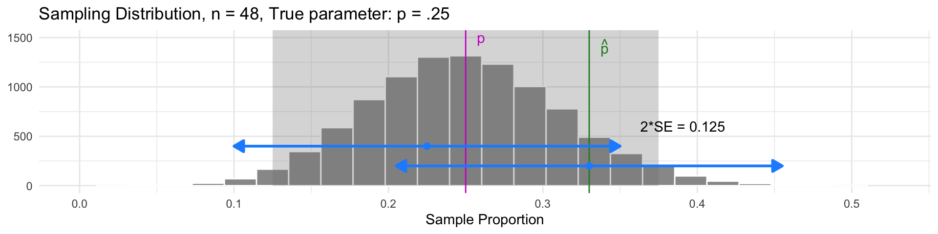
- Samples with \(\widehat{p}\) in the gray region have intervals that also contain the parameter \(p\)
Interval Estimates
Idea: Build an interval centered at the sample statistic, with a margin of error of \(2\cdot SE\):
\[
\widehat{p} \pm 2\cdot \textrm{SE}
\]
- This interval will contain the parameter \(p\) in 95% of samples!
- Samples with \(\widehat{p}\) outside the gray region have intervals that don’t contain \(p\)
Interval Estimates
Idea: Build an interval centered at the sample statistic, with a margin of error of \(2\cdot SE\):
\[
\widehat{p} \pm 2\cdot \textrm{SE}
\]
- This interval will contain the parameter \(p\) in 95% of samples!
- But 95% of all samples will have intervals that do contain \(p\)
Confidence levels
On the previous slide, 95% of confidence intervals contained the true parameter, \(p\).
Thus, we call each interval estimate a 95% confidence interval.
Here, 95% is our confidence level: The success rate for our estimation technique.
- e.g., The pizza interval \(0.33 \pm 0.13\) has confidence level of 95%
The confidence level corresponds to the percentage of samples that would yield a corresponding confidence interval containing the true value of the parameter.
Recap: Confidence Intervals
Confidence intervals consist of 1. an interval estimate and 2. a confidence level.
In our pizza party sample, we estimated the true proportion of vegetarian pizza-eaters was between \(0.20\) and \(0.46\), with \(95\%\) confidence.
What does “95% confidence” mean?
- It’s the success rate of the process
- For 95% of all samples, the interval we construct will actually contain the parameter.
Worth emphasizing: it’s the success rate of The Process, NOT the specific interval you calculated in your sample.
- The parameter is either in your interval, or it’s not – there’s no success rate there!
Think-Pair-Share
Q: What’s the difference between these two interpretations of a 95% confidence interval?
For 95% of all samples, the interval we construct will actually contain the parameter.
For a given interval, there is a 95% chance that the parameter will fall in the interval.
Think-Pair-Share (Answer)
Q: What’s the difference between these two interpretations of a 95% confidence interval?
For 95% of all samples, the interval we construct will actually contain the parameter.
For a given interval, there is a 95% chance that the parameter will fall in the interval.
The first one is accurate! 95% confidence refers to the accuracy of the process
The second one is wrong, an easy mistake to make!! It confuses probability of the process with a deterministic outcome. Our sample statistic “moves” with sampling variability - the parameter does not.
Interval Width and Sample Size (\(n\))
Idea: Build a 95% confidence interval centered at the sample statistic, with a margin of error of \(2\cdot SE\): \[
\widehat{p} \pm \underbrace{2\cdot \textrm{SE}}_{\text{Margin of Error}}
\]
This interval’s width is determined by the Standard Error (SE).
Reminder: The SE is the standard deviation of the sampling distribution.
Q: What do we know about the SE as the sample size (\(n\)) increases?
Q: What does this imply about the interval’s width as the sample size (\(n\)) increases?
- The SE gets smaller as \(n\) increases!
- Our interval becomes narrower as \(n\) increases!
Interval Width and Confidence Level
Idea: Build an 95% confidence interval centered at the sample statistic, with a margin of error of \(2\cdot SE\): \[
\widehat{p} \pm \underbrace{2\cdot \textrm{SE}}_{\text{Margin of Error}}
\]
Chose \(\text{Margin of Error} = 2*SE\) because 95% of sample statistics fall within \(2*SE\) of the parameter (in sampling distribution).
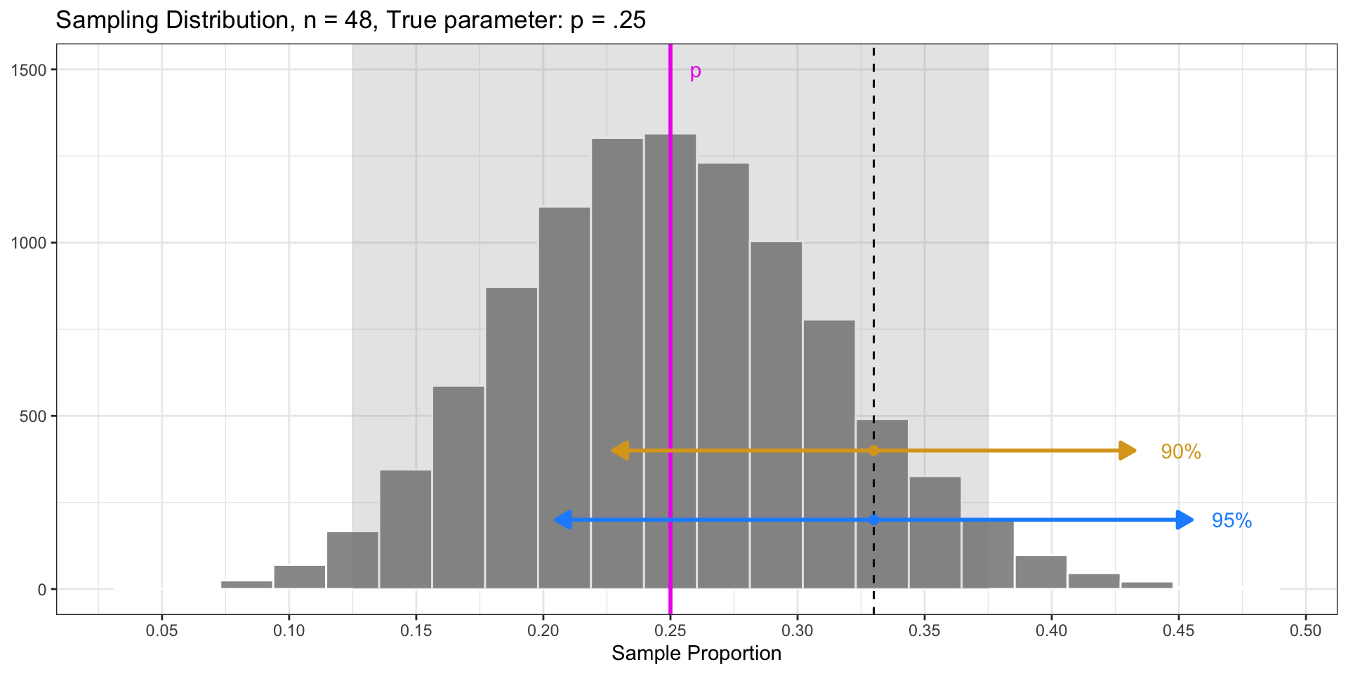
Fun Fact: 90% of sample statistics fall within \(1.64*SE\) of the parameter.
- Q: What would happen if we did the following interval? \[
\widehat{p} \pm 1.64*\textrm{SE}
\]
- We would get a 90% confidence interval!
- This interval is narrower, but has a lower “success” rate! For 90% of all samples, the interval will contain the parameter.
Interval Width and Confidence Level
Problems(?) with Confidence Intervals
Let’s say we’re working with 95% confidence intervals
- Problem 1: We only have 1 sample, and we don’t know if it belongs to the 95% of “good” samples, or the 5% of “bad” ones
- Consolation: If I go through life constructing 95% confidence intervals, I will be right about 95% of the time
- That’s not bad!
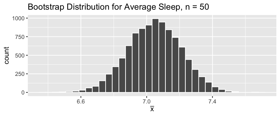
- Problem 2: To make a confidence interval, we need the sampling distribution in order to compute the standard error. But in practice, we (often) don’t have direct access to this.
- Solution: approximate the sampling distribution via bootstrapping!