Sampling and Bootstrap Distributions
Megan Ayers
Math 141 | Spring 2026
Friday, Week 6
Question 1
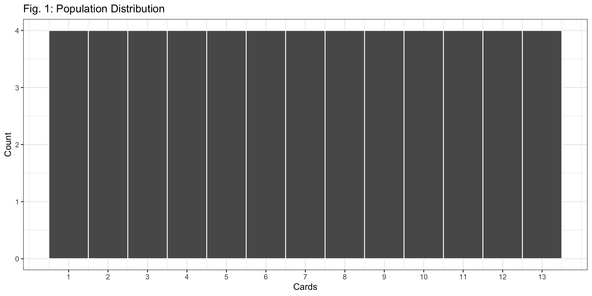
Q1: In Figure 1, why is the height of each bar 4? Describe this distribution.
There are four cards of each value in a deck.
The distribution has a “flat” shape, centered at 7 (mean = 7 and median = 7).
The distribution has a “large” spread. Standard Deviation: 3.78
Question 3
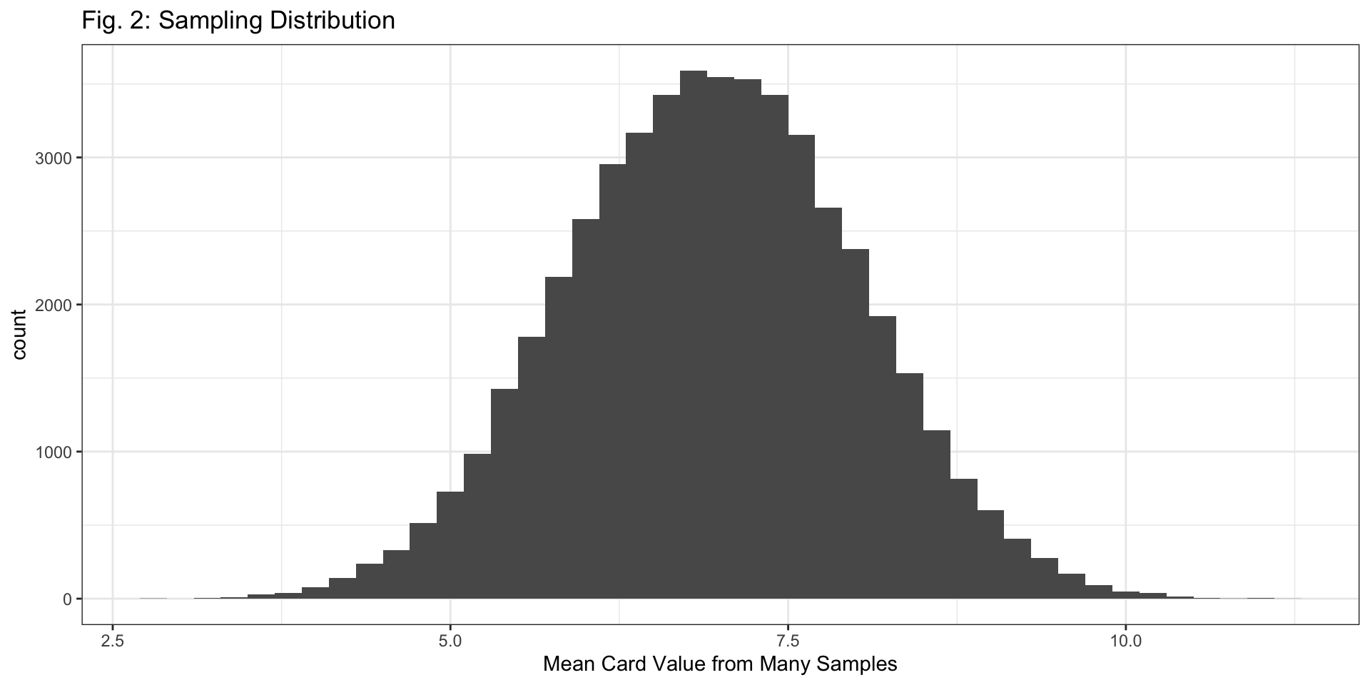
Q3: Based on the code above, how many cards are in each sample? How many different samples did we take to create the sampling distribution in Figure 2?
There are 10 cards in each sample, since
size = 10.We took 50,000 different samples, since
reps = 50000.
Question 4
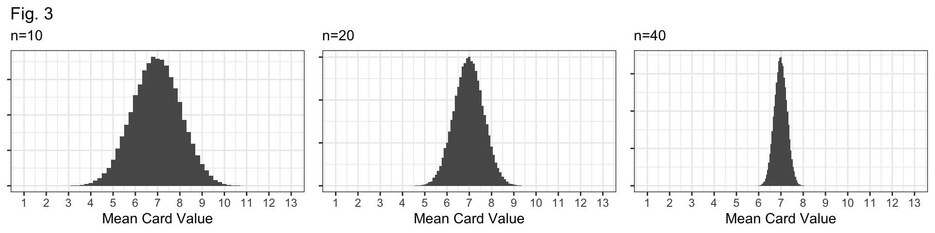
Q4: Figure 3 (below) displays sampling distributions for samples of size n=10, n=20, and n=40. How are they similar and how are they different? Why do larger samples have sampling distributions with less variability?
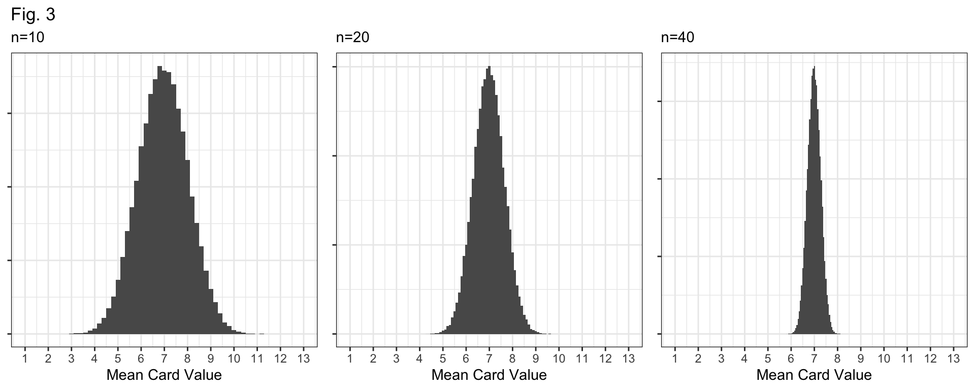
Bell-shaped and centered at the true mean, 7.
They differ in their spread: \(n=10\) distribution has the largest standard error; the \(n=40\) distribution has the smallest standard error.
Question 4
Q4: Figure 3 (below) displays sampling distributions for samples of size n=10, n=20, and n=40. How are they similar and how are they different? Why do larger samples have sampling distributions with less variability?

Why? If our sample size (\(n\)) is larger, we have more data and our sample should be “more representative” of the population.
i.e., more data means a better glimpse at the true population, and better guesses about the population mean!
Question 7
single_sample %>% ungroup() %>% select(cards) %>%
  rep_sample_n(size = 10, replace = TRUE, reps = 20000) %>%
  group_by(replicate) %>%
  summarize(x_bar = mean(cards)) %>%
  ggplot(aes(x = x_bar)) + geom_histogram(binwidth = 0.1) +
  labs(x = "Mean Card Value Based on Samples of Size 10",
       title = "Fig. 4: Bootstrap Distribution") +
  theme_bw() +
  scale_x_continuous(breaks = 1:13, limits = c(1, 13))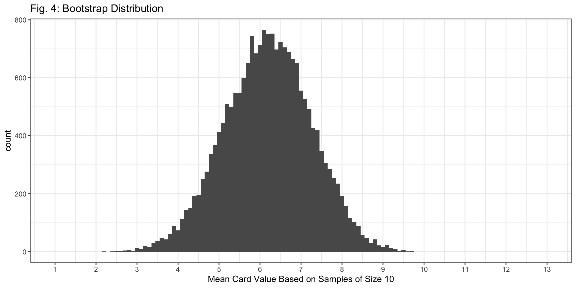
Q7: Based on the code above, how many bootstrap samples are we taking to create the bootstrap distribution?
- 20,000 bootstrap samples because
reps=20000.
Question 8
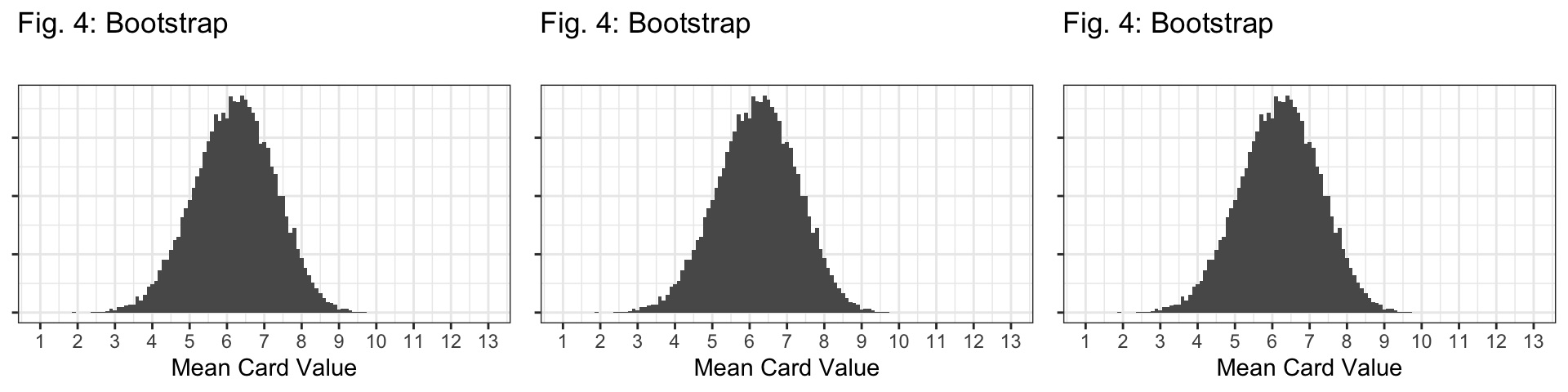
Q8: Which sampling distribution looks most like the bootstrap distribution in Figure 4? How specifically is it similar or different? Consider the shape, center, and spread of each distibution.
Question 8


The \(n=10\) sampling distribution!
Question 8


Shape: All distributions look bell-shaped, so this doesn’t distinguish them at all.
Question 8


Center: Bootstrap is centered at the sample mean (6.2); all sampling distributions are centered at the population mean (7).
Question 8


Spread: The spread of the bootstrap distribution looks similar to the spread of the sampling distribution with \(n=10\).