Linear Models V

Megan Ayers

Math 141 | Spring 2026
Wednesday, Week 5

Goals for Today

• Learning Check
• Regression with many variables
• Adjusted \(R^2\) and model selection
• Multicollinearity
• Application of Multiple Linear Regression

Learning check handout

Linear Regression

Model Form:

\[ \begin{align} y &= \beta_0 + \beta_1 x_1 + \beta_2 x_2 + \cdots + \beta_p x_p + \epsilon \end{align} \]

Linear regression is a flexible class of models that allow for:

• Both quantitative and categorical explanatory variables.

• Multiple explanatory variables.

• Transformed explanatory variables.

• BUT the response variable is quantitative.

More time with the palmerpenguins!

Recap: Regression with the penguins so far

One Quantitative Variable

library(palmerpenguins)
library(moderndive)
mod <- lm(bill_length_mm ~ bill_depth_mm,
          data = penguins)
get_regression_table(mod) %>% select(term, estimate)

# A tibble: 2 × 2
  term          estimate
  <chr>            <dbl>
1 intercept        55.1 
2 bill_depth_mm    -0.65

One Categorical Variable

mod <- lm(bill_length_mm ~ species,
          data = penguins)
get_regression_table(mod) %>% select(term, estimate)

# A tibble: 3 × 2
  term               estimate
  <chr>                 <dbl>
1 intercept             38.8 
2 species: Chinstrap    10.0 
3 species: Gentoo        8.71

Equal Slopes Model

mod <- lm(bill_length_mm ~ species + bill_depth_mm,
          data = penguins)
get_regression_table(mod) %>% select(term, estimate)

# A tibble: 4 × 2
  term               estimate
  <chr>                 <dbl>
1 intercept             13.2 
2 species: Chinstrap     9.94
3 species: Gentoo       13.4 
4 bill_depth_mm          1.39

Different Slopes Model

mod <- lm(bill_length_mm ~ species*bill_depth_mm,
          data = penguins)
get_regression_table(mod) %>% select(term, estimate)

# A tibble: 6 × 2
  term                             estimate
  <chr>                               <dbl>
1 intercept                          23.1  
2 species: Chinstrap                 -9.64 
3 species: Gentoo                    -5.84 
4 bill_depth_mm                       0.857
5 species: Chinstrap:bill_depth_mm    1.06 
6 species: Gentoo:bill_depth_mm       1.16 

This time: Regression with multiple quantitative predictors

ggplot(penguins, aes(x = body_mass_g, y = bill_length_mm)) +
  geom_point()

ggplot(penguins, aes(x = bill_depth_mm, y = bill_length_mm)) +
  geom_point()

\[ y = \beta_0 + \beta_1x_{\textrm{Bill Depth}} + \beta_2 x_{\textrm{Body Mass}} + \epsilon \]

This time: Regression with multiple quantitative predictors

In R:

mod <- lm(bill_length_mm ~ bill_depth_mm + body_mass_g, penguins)
get_regression_table(mod)

# A tibble: 3 × 7
  term          estimate std_error statistic p_value lower_ci upper_ci
  <chr>            <dbl>     <dbl>     <dbl>   <dbl>    <dbl>    <dbl>
1 intercept       23.3       3.27       7.14   0       16.9     29.7  
2 bill_depth_mm    0.163     0.137      1.19   0.234   -0.106    0.432
3 body_mass_g      0.004     0         12.6    0        0.004    0.005

Visualizing the best fit plane

options(rgl.useNULL = TRUE)
options(rgl.printRglwidget = TRUE)
library(rgl)
plot3d(x = penguins$bill_depth_mm, y = penguins$body_mass_g, 
       z = penguins$bill_length_mm, type = "s", col = "goldenrod", size = 1)
planes3d(a = coef(mod)[2], b = coef(mod)[3], c=-1, d = coef(mod)[1], alpha = .5)

Least Squares and Prediction

• Still minimizing the sum of squared residuals (from the plane)
• Still predict like usual

pred_dat <- data.frame(bill_depth_mm = c(16, 18),
                       body_mass_g = c(4000, 5000))
predict(mod, pred_dat)

       1        2 
42.87888 47.44527 

Model Building Guidance

Should we always include an interaction term? How many variables should I include?

Guiding Principle: Occam’s Razor for Modeling

“All other things being equal, simpler models are to be preferred over complex ones.” – ModernDive

Guiding Principle: Consider your modeling goals.

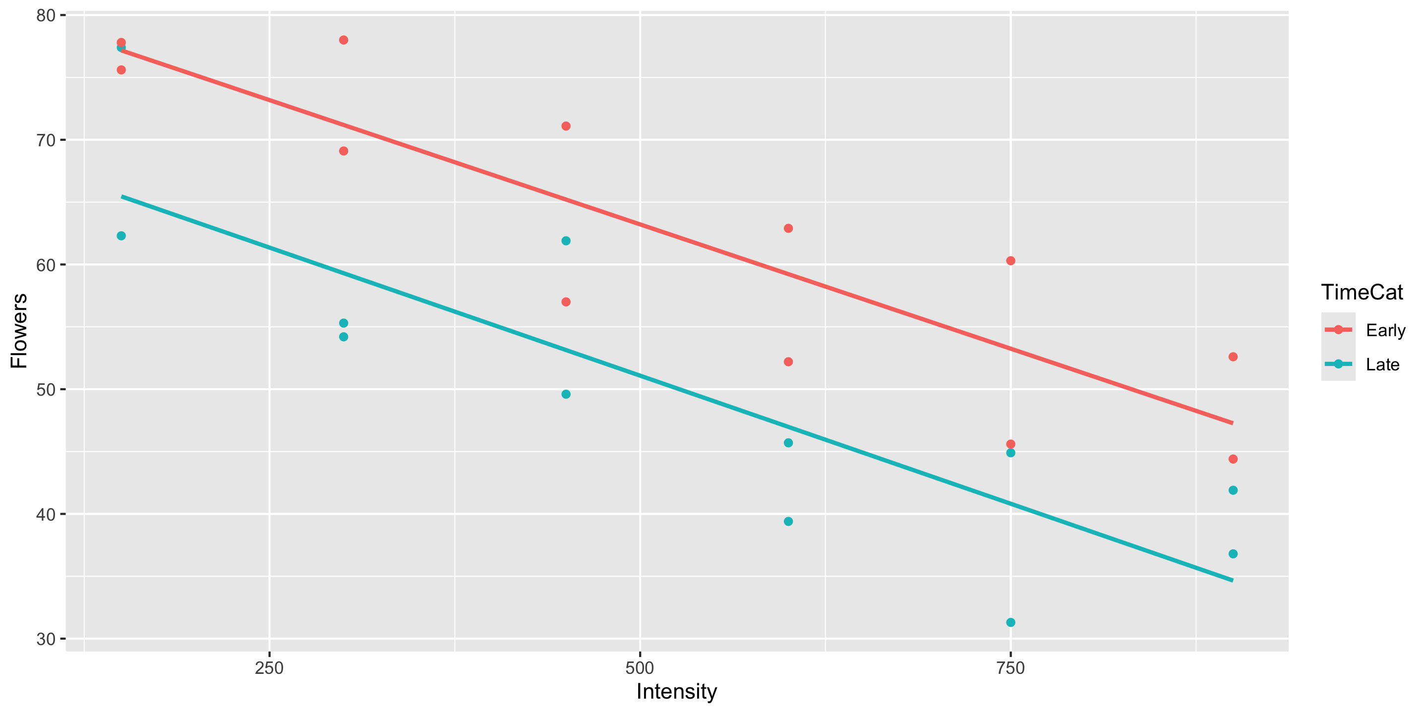
• The equal slopes model allows us to control for the intensity of the light and then see the impact of being in the early or late timing groups on the number of flowers.

• Later in the course will learn statistical procedures for determining whether or not a particular term should be included in the model.

What if I want to include many explanatory variables??

Model Building Guidance

We often have several potential explanatory variables. How do we determine which to include in the model and in what form?

Guiding Principle: Include explanatory variables that attempt to explain different aspects of the variation in the response variable.

Example: Movie Ratings

library(tidyverse)
library(moderndive)
movies <- read_csv("https://www.lock5stat.com/datasets2e/HollywoodMovies.csv")

# Restrict our attention to dramas, horrors, and actions
movies2 <- movies %>%
  filter(Genre %in% c("Drama", "Horror", "Action")) %>%
  drop_na(Genre, AudienceScore, RottenTomatoes)
glimpse(movies2)

Rows: 313
Columns: 16
$ Movie            <chr> "Spider-Man 3", "Transformers", "Pirates of the Carib…
$ LeadStudio       <chr> "Sony", "Paramount", "Disney", "Warner Bros", "Warner…
$ RottenTomatoes   <dbl> 61, 57, 45, 60, 20, 79, 35, 28, 41, 71, 95, 42, 18, 2…
$ AudienceScore    <dbl> 54, 89, 74, 90, 68, 86, 55, 56, 81, 52, 84, 55, 70, 6…
$ Story            <chr> "Metamorphosis", "Monster Force", "Rescue", "Sacrific…
$ Genre            <chr> "Action", "Action", "Action", "Action", "Action", "Ac…
$ TheatersOpenWeek <dbl> 4252, 4011, 4362, 3103, 3778, 3408, 3959, 3619, 2911,…
$ OpeningWeekend   <dbl> 151.1, 70.5, 114.7, 70.9, 49.1, 33.4, 58.0, 45.3, 19.…
$ BOAvgOpenWeekend <dbl> 35540, 17577, 26302, 22844, 12996, 9791, 14663, 12541…
$ DomesticGross    <dbl> 336.53, 319.25, 309.42, 210.61, 140.13, 134.53, 131.9…
$ ForeignGross     <dbl> 554.34, 390.46, 654.00, 245.45, 117.90, 249.00, 157.1…
$ WorldGross       <dbl> 890.87, 709.71, 963.42, 456.07, 258.02, 383.53, 289.0…
$ Budget           <dbl> 258.0, 150.0, 300.0, 65.0, 140.0, 110.0, 130.0, 110.0…
$ Profitability    <dbl> 345.30, 473.14, 321.14, 701.64, 184.30, 348.66, 222.3…
$ OpenProfit       <dbl> 58.57, 47.00, 38.23, 109.08, 35.07, 30.36, 44.62, 41.…
$ Year             <dbl> 2007, 2007, 2007, 2007, 2007, 2007, 2007, 2007, 2007,…

Example: Movie Ratings

library(GGally)
movies2 %>%
  select(RottenTomatoes, AudienceScore, OpeningWeekend, DomesticGross, Genre) %>%
  ggpairs()

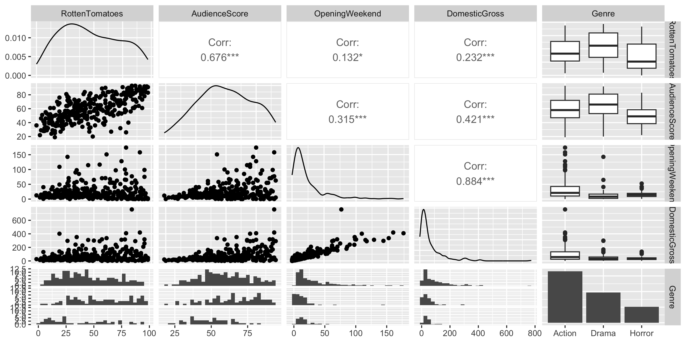
• Multicollinearity: when explanatory variables are highly correlated with one another. Multicollinearity often results in coefficients that are distorted in erroneous ways!

• Q: Do any of these variables seem to be measuring the same thing?

Model Building Guidance

We often have several potential explanatory variables. How do we determine which to include in the model and in what form?

Guiding Principle: Include explanatory variables that attempt to explain different aspects of the variation in the response variable.

mod_movies <- lm(RottenTomatoes ~ AudienceScore + Genre + DomesticGross, data = movies2)
get_regression_table(mod_movies)

# A tibble: 5 × 7
  term          estimate std_error statistic p_value lower_ci upper_ci
  <chr>            <dbl>     <dbl>     <dbl>   <dbl>    <dbl>    <dbl>
1 intercept      -12.5       4.08     -3.06    0.002  -20.5     -4.44 
2 AudienceScore    0.975     0.072    13.6     0        0.834    1.12 
3 Genre: Drama     6.12      2.64      2.31    0.021    0.916   11.3  
4 Genre: Horror    2.06      3.14      0.655   0.513   -4.12     8.24 
5 DomesticGross   -0.006     0.015    -0.431   0.667   -0.035    0.023

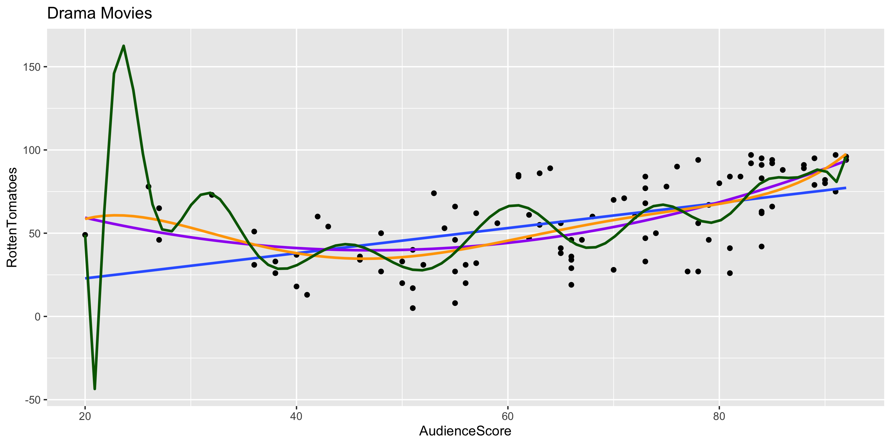
Transformations: Model Building Guidance

What degree of polynomial should I include in my model?

Guiding Principle: Capture the general trend, not the noise.

\[ \begin{align} y &= f(x) + \epsilon \\ y &= \mbox{TREND} + \mbox{NOISE} \end{align} \]

Model Building Guidance

Suppose I built 3 different models. Which is best?

mod1 <- lm(RottenTomatoes ~ AudienceScore, data = movies2)
mod2 <- lm(RottenTomatoes ~ AudienceScore + Genre, data = movies2)
mod3 <- lm(RottenTomatoes ~ AudienceScore + Genre + DomesticGross, data = movies2)

• Big question! Take Math 243: Statistical Learning to learn systematic model selection techniques.

• We will explore one approach. (But there are many possible approaches!)

Comparing Models with \(R^2\)

Strategy: Compute the \(R^2\) value for each model and pick the one with the highest \(R^2\).

mod1 <- lm(RottenTomatoes ~ AudienceScore, data = movies2)
mod2 <- lm(RottenTomatoes ~ AudienceScore + Genre, data = movies2)
mod3 <- lm(RottenTomatoes ~ AudienceScore + Genre + DomesticGross, data = movies2)

get_regression_summaries(mod1) %>% select(r_squared)

# A tibble: 1 × 1
  r_squared
      <dbl>
1     0.457

get_regression_summaries(mod2) %>% select(r_squared)

# A tibble: 1 × 1
  r_squared
      <dbl>
1     0.469

get_regression_summaries(mod3) %>% select(r_squared)

# A tibble: 1 × 1
  r_squared
      <dbl>
1     0.469

Strategy: Compute the \(R^2\) value for each model and pick the one with the highest \(R^2\).

get_regression_summaries(mod1) %>% select(r_squared)

# A tibble: 1 × 1
  r_squared
      <dbl>
1     0.457

get_regression_summaries(mod2) %>% select(r_squared)

# A tibble: 1 × 1
  r_squared
      <dbl>
1     0.469

get_regression_summaries(mod3) %>% select(r_squared)

# A tibble: 1 × 1
  r_squared
      <dbl>
1     0.469

Problem: As we add predictors, the \(R^2\) value will only increase.

Guiding Principle: Occam’s Razor for Modeling

“All other things being equal, simpler models are to be preferred over complex ones.” – ModernDive

Comparing Models with the Adjusted \(R^2\)

New Measure of quality: Adjusted \(R^2\) (Coefficient of Determination)

\[\begin{align*} \mbox{adj} R^2 &= 1- \frac{\sum (y - \widehat{y})^2}{\sum (y - \bar{y})^2} \left(\frac{n - 1}{n - p - 1} \right) \end{align*}\]

where \(p\) is the number of explanatory variables in the model.

• Now we will penalize larger models.

• Strategy: Compute the adjusted \(R^2\) value for each model and pick the one with the highest adjusted \(R^2\).

Strategy: Compute the adjusted \(R^2\) value for each model and pick the one with the highest adjusted \(R^2\).

mod1 <- lm(RottenTomatoes ~ AudienceScore, data = movies2)
mod2 <- lm(RottenTomatoes ~ AudienceScore + Genre, data = movies2)
mod3 <- lm(RottenTomatoes ~ AudienceScore + Genre + DomesticGross, data = movies2)

get_regression_summaries(mod1) %>% select(r_squared, adj_r_squared)

# A tibble: 1 × 2
  r_squared adj_r_squared
      <dbl>         <dbl>
1     0.457         0.455

get_regression_summaries(mod2) %>% select(r_squared, adj_r_squared)

# A tibble: 1 × 2
  r_squared adj_r_squared
      <dbl>         <dbl>
1     0.469         0.464

get_regression_summaries(mod3) %>% select(r_squared, adj_r_squared)

# A tibble: 1 × 2
  r_squared adj_r_squared
      <dbl>         <dbl>
1     0.469         0.462

Case Study: Home Prices in King County, WA

We’ll consider : Sale price (response); and square footage, above-ground square footage, and number of bedrooms (potential explanatory variables). Check out the exploratory plots below:

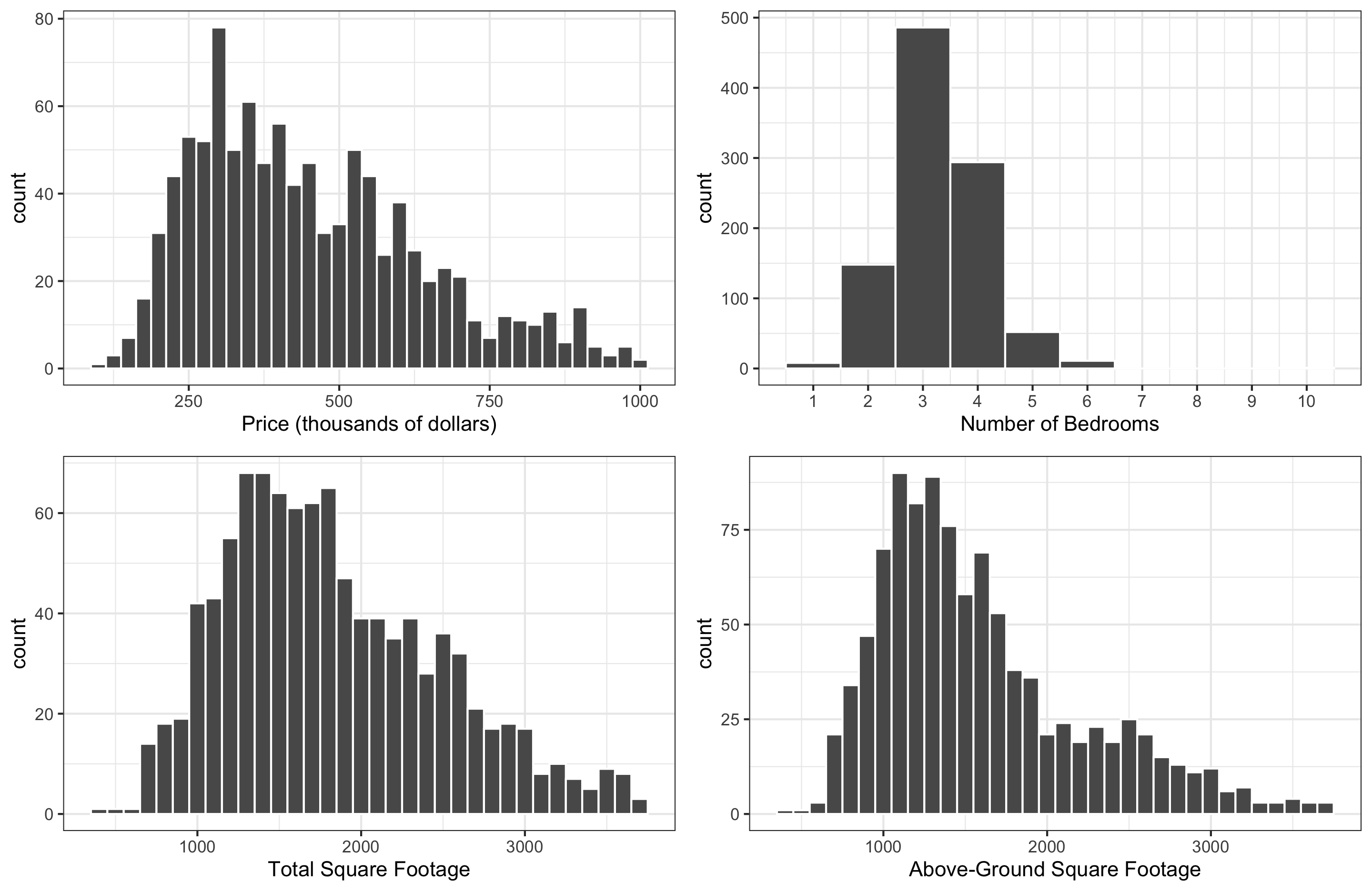
• Q: How would you describe the distribution of price?

• Q: What do you expect the relationship between price and bedrooms to be like?

Exploration, Multicollinearity

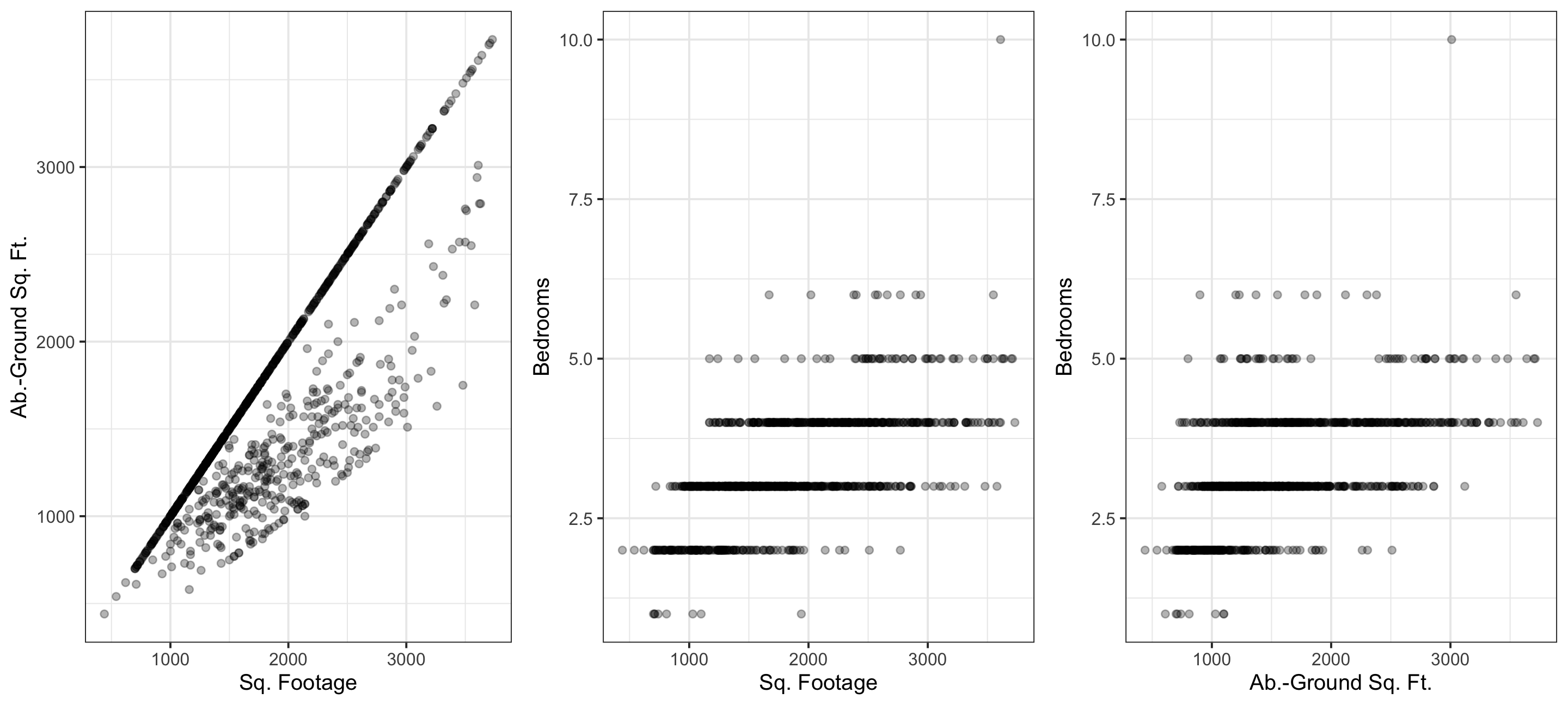
• Multicollinearity: when explanatory variables are highly correlated with one another. Multicollinearity often results in coefficients that are distorted in erroneous ways! We want to avoid this (some correlation is okay!)

• Q: Which pair of explanatory variables suffers most from multicollinearity?

Model Estimation

# A tibble: 3 × 7
  term        estimate std_error statistic p_value lower_ci upper_ci
  <chr>          <dbl>     <dbl>     <dbl>   <dbl>    <dbl>    <dbl>
1 intercept    197.        19.4      10.1    0      159.     235.   
2 sqft_living    0.177      0.01     18.4    0        0.158    0.196
3 bedrooms     -21.6        7.27     -2.97   0.003  -35.9     -7.34 

• Q: What is the equation, including coefficient values, for the estimated model?

\[ \widehat{\text{price}} = 197 + 0.177*\text{sqrt_living} - 21.6*\text{bedrooms} \]

• Q: How should interpret the intercept coefficient in our model?
  • When sqrt_living and bedrooms are both 0, we expect/predict price to be $197,000 on average.
• Q: The coefficient for Bedrooms? Does this match your expectation?
  • When the number of bedrooms increases by 1, we expect/predict price to decrease by $21,600 on average, holding sqft_living constant.

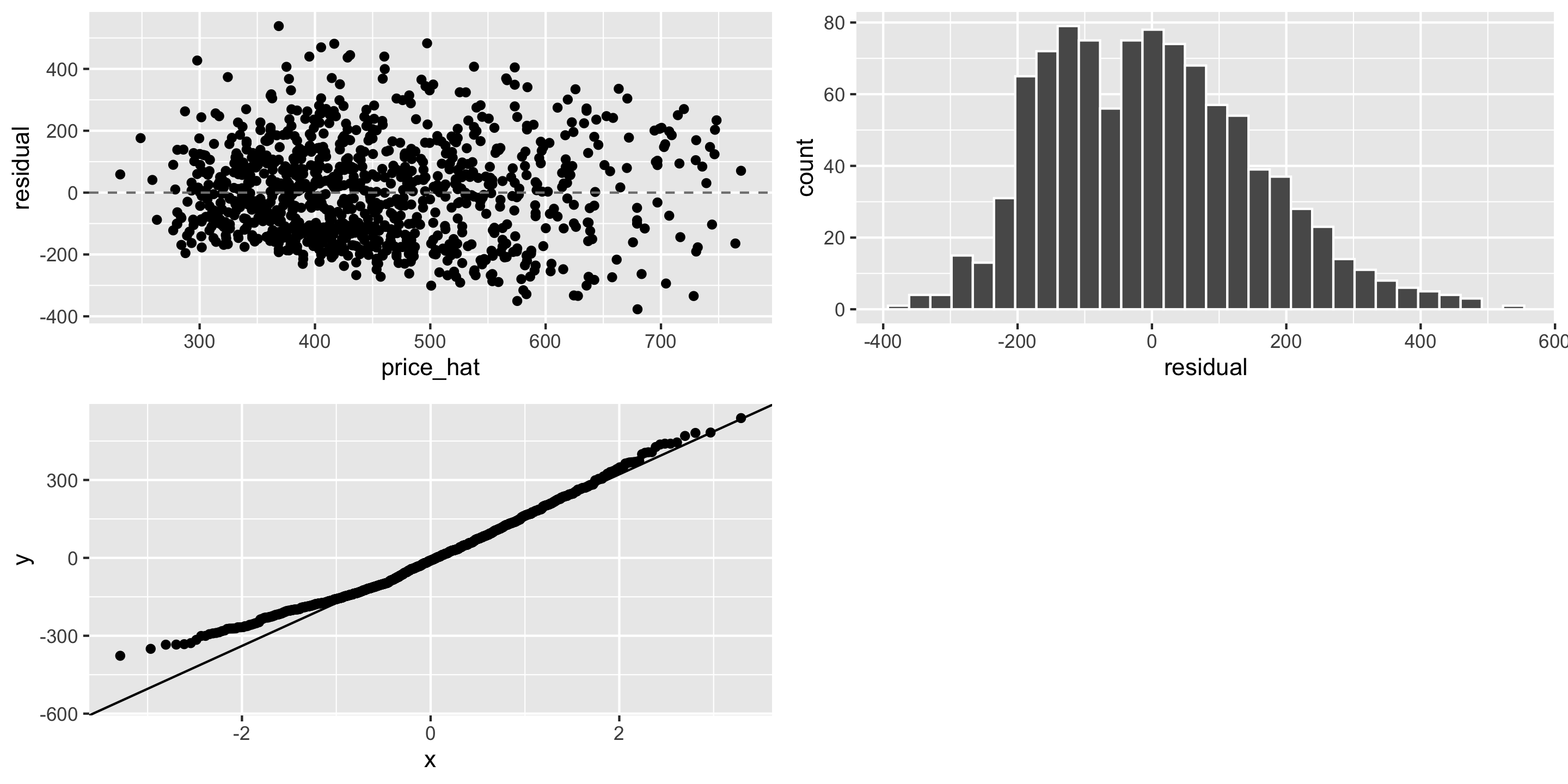
LINE Assumptions

Adjusted \(R^2\)

What’s the adjusted \(R^2\) of our model?

get_regression_summaries(mod)[, c("r_squared", "adj_r_squared")]

# A tibble: 1 × 2
  r_squared adj_r_squared
      <dbl>         <dbl>
1     0.314         0.313

Not super close to 1. Compare to a simpler model:

small_mod <- lm(price ~ bedrooms, data = house)
get_regression_summaries(small_mod)[, c("r_squared", "adj_r_squared")]

# A tibble: 1 × 2
  r_squared adj_r_squared
      <dbl>         <dbl>
1     0.082         0.081

Compare to a much bigger model with additional variables:

big_mod <- lm(price ~ bedrooms + bathrooms + sqft_living + sqft_above + sqft_lot + 
                view + condition + yr_built, data = house)
get_regression_summaries(big_mod)[, c("r_squared", "adj_r_squared")]

# A tibble: 1 × 2
  r_squared adj_r_squared
      <dbl>         <dbl>
1     0.434         0.429

Developing Linear Models

• Key components that we’ve learned about over the last 5 lectures:

  • Determining the response variable and the potential explanatory variable(s)
  • Writing out the model form and understanding what the terms represent in context
  • Building and visualizing linear regression models in R
  • Validating model assumptions with diagnostic plots
  • Comparing different potential models

Next time

• Sampling distributions!