  Time  n
1    1 12
2    2 12
Linear Models IV: Multiple Regression
Megan Ayers
Math 141 | Spring 2026
Monday, Week 5
Example
Meadowfoam is a plant that grows in the Pacific Northwest and is harvested for its seed oil. In a randomized experiment, researchers at Oregon State University looked at how two light-related factors influenced the number of flowers per meadowfoam plant, the primary measure of productivity for this plant. The two light measures were light intensity (in mmol/ \(m^2\) /sec) and the timing of onset of the light (early or late in terms of photo periodic floral induction).

Response variable?
Explanatory variables?
Model Form?
Visualizing the Data
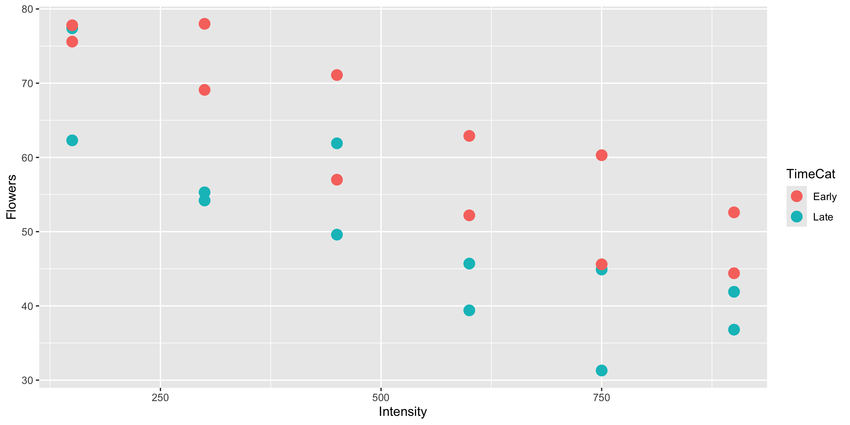
Q: How does this plot help us intuit what \(\widehat{\beta}_0\), \(\widehat{\beta}_1\), and \(\widehat{\beta}_2\) might be?
Why don’t I have to include
data =andmapping =in myggplot()layer?
Appropriateness of Model Form
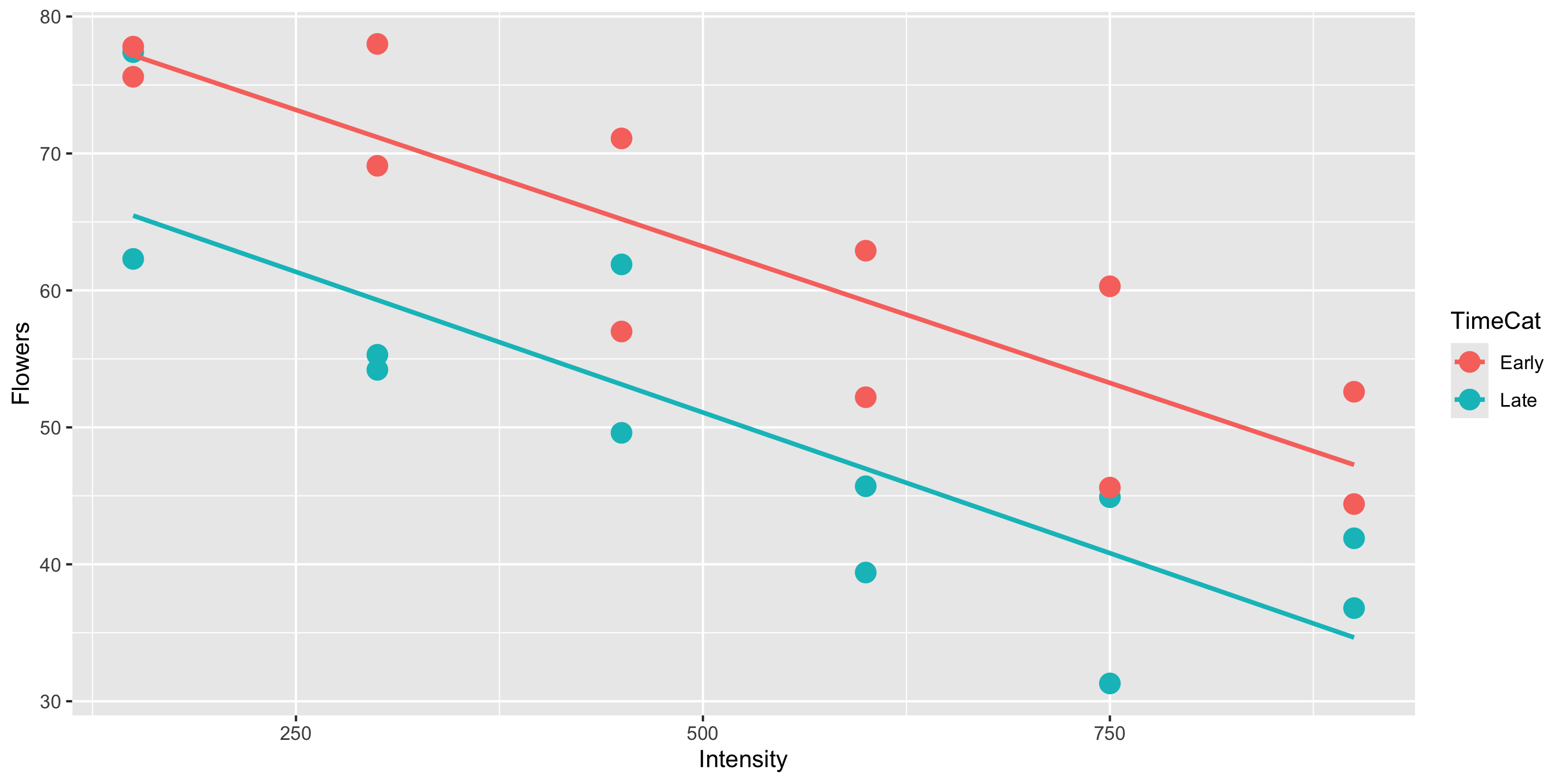
Is the assumption of equal slopes reasonable here?
Returning to the Palmer Penguins
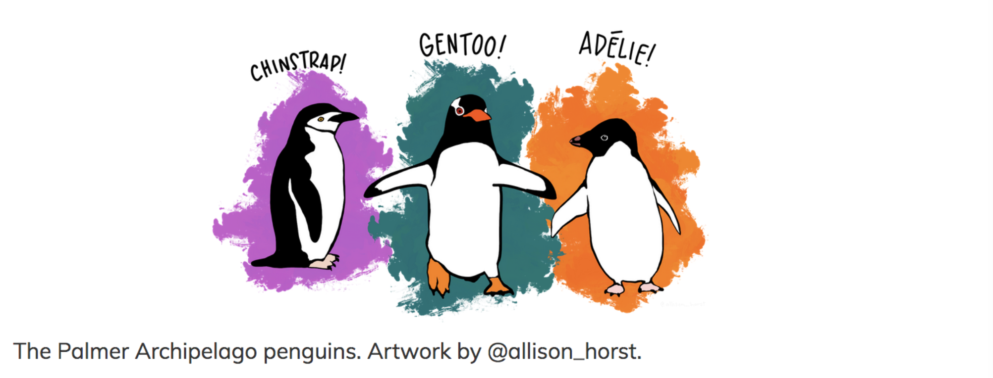
Last time:
We predicted a penguin’s bill length based on their species.
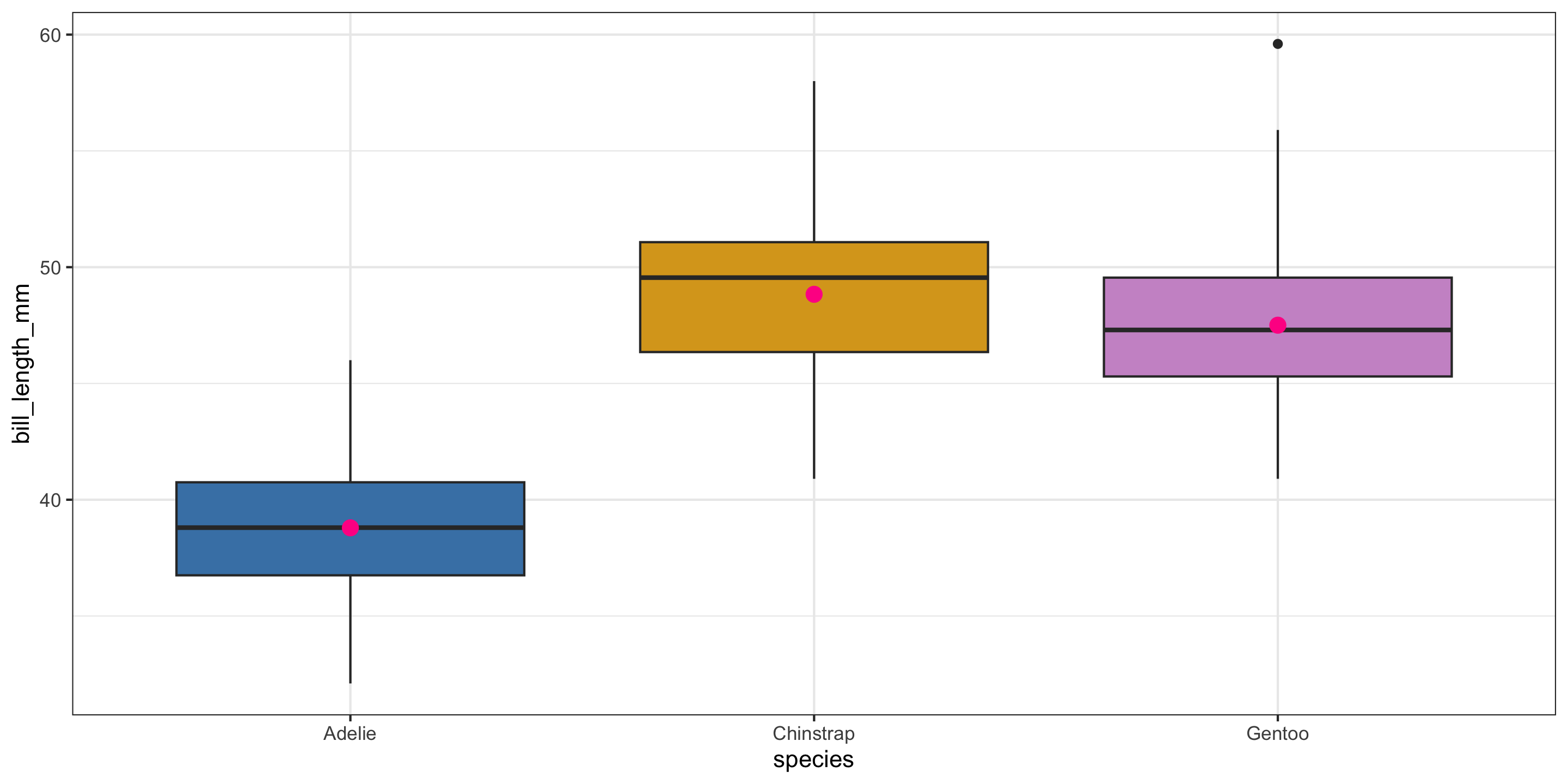
- Pink dots represent the mean value in each group.
- For the single categorical variable model, those pink dots are the predicted values for each group.
This time:
We’ll incorporate bill depth for prediction!
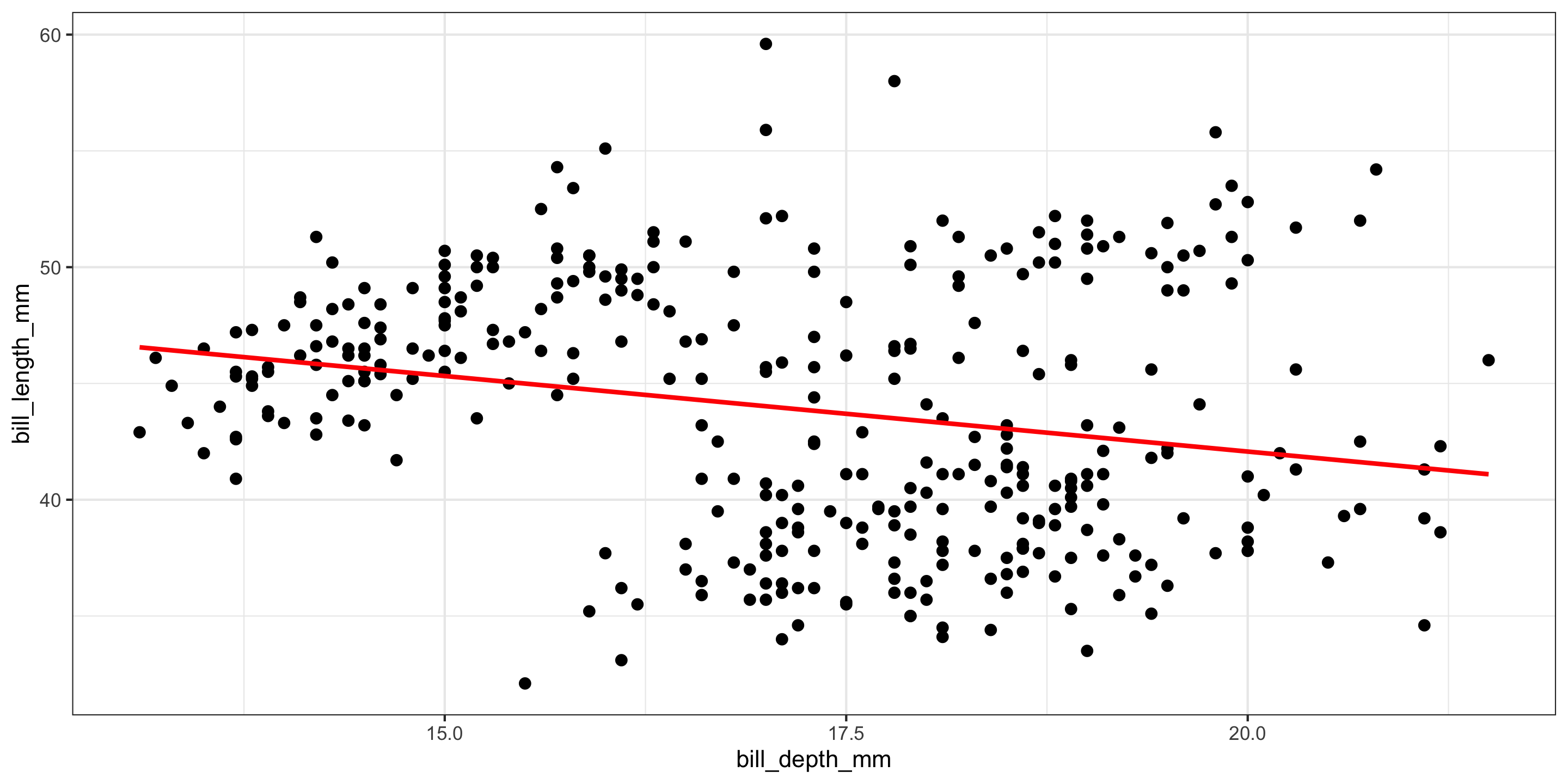
- A moderate negative relationship between bill length and bill depth!
- Does this make sense?
What if we include both explanatory variables?
ggplot(penguins, aes(x = bill_depth_mm,
                     y = bill_length_mm,
                     color = species)) +
  geom_point(size = 2) +
  geom_smooth(inherit.aes = FALSE,
              mapping = aes(x = bill_depth_mm,
                            y = bill_length_mm),
              method = "lm", se = FALSE,
              color = "red") +
  geom_parallel_slopes(se = FALSE) +
  scale_color_manual(values = c("steelblue",
                               "goldenrod",
                               "plum3")) +
  theme_bw() +
  theme(legend.position = "bottom")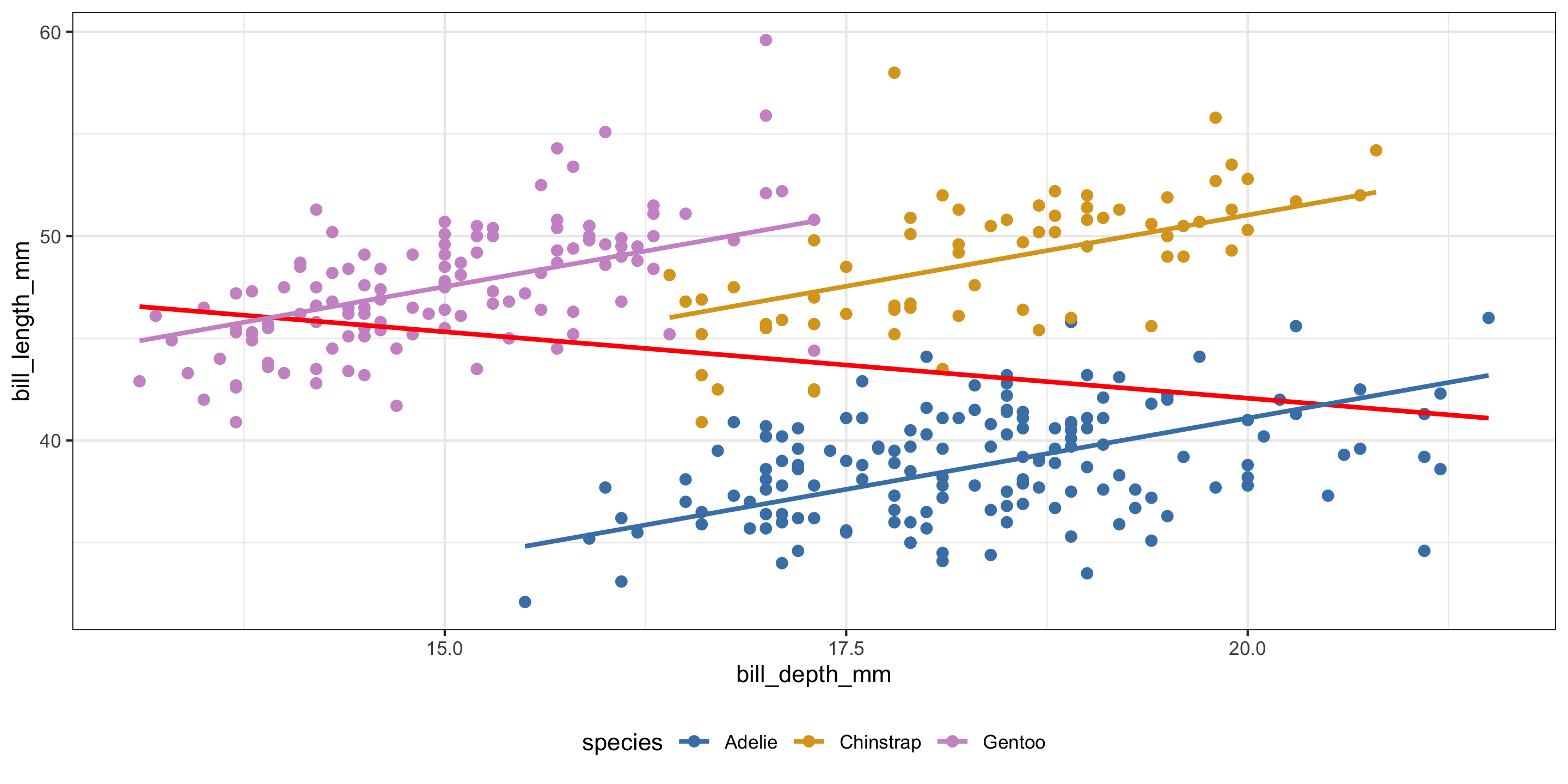
- Negative relationships between bill depth and bill length overall.
- Positive relationships between bill depth and bill length when accounting for species!
- What is going on here??
- This is a case of Simpson’s Paradox.
Returning to our MLR model
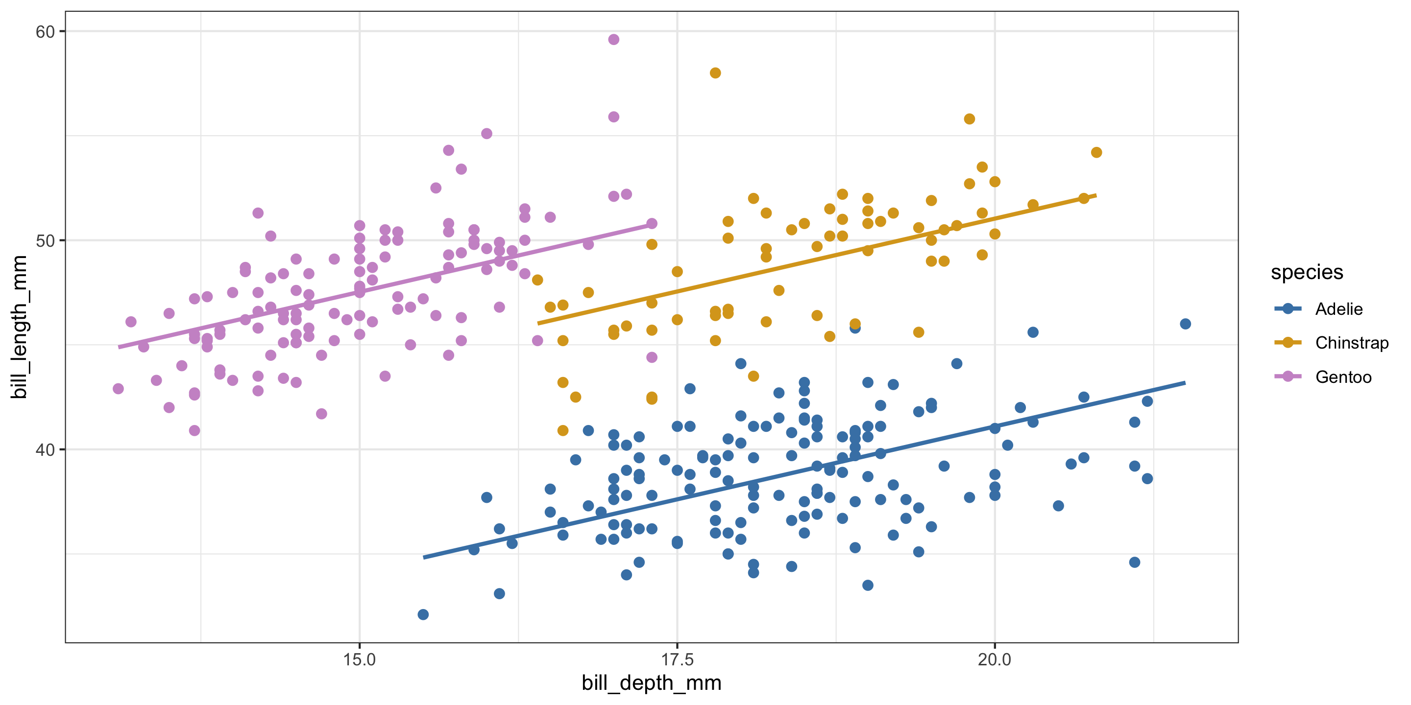
Are equal slopes a reasonable assumption here?
Different Slopes Model

Equal slopes models force the relationship between quantitative predictors and the response variable to be the same for each group in the model.
In contrast, different slopes models allow for different relationships between quantitative predictors and the response variable for each group in the model.
How can we allow our model to have different slopes?
Exploring the Data
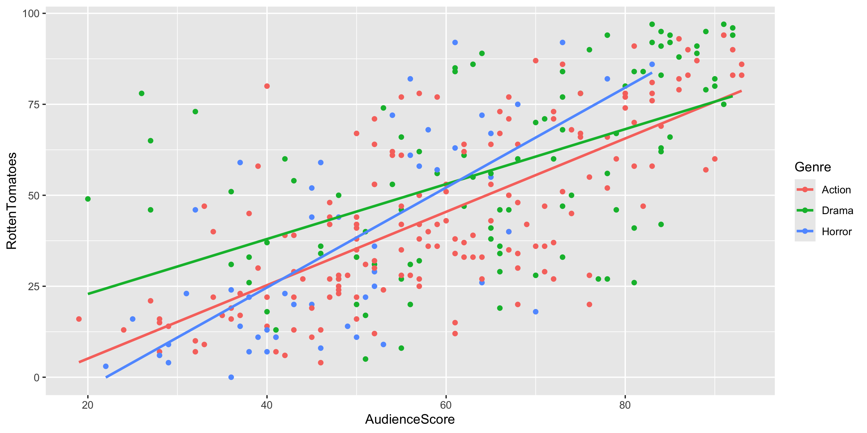
- Q: What do the trends suggest, would it make sense to include interaction terms in the model?
- Q: Does anyone spot a curved relationship for one of the genres?
Adding a Curve to your Scatterplot
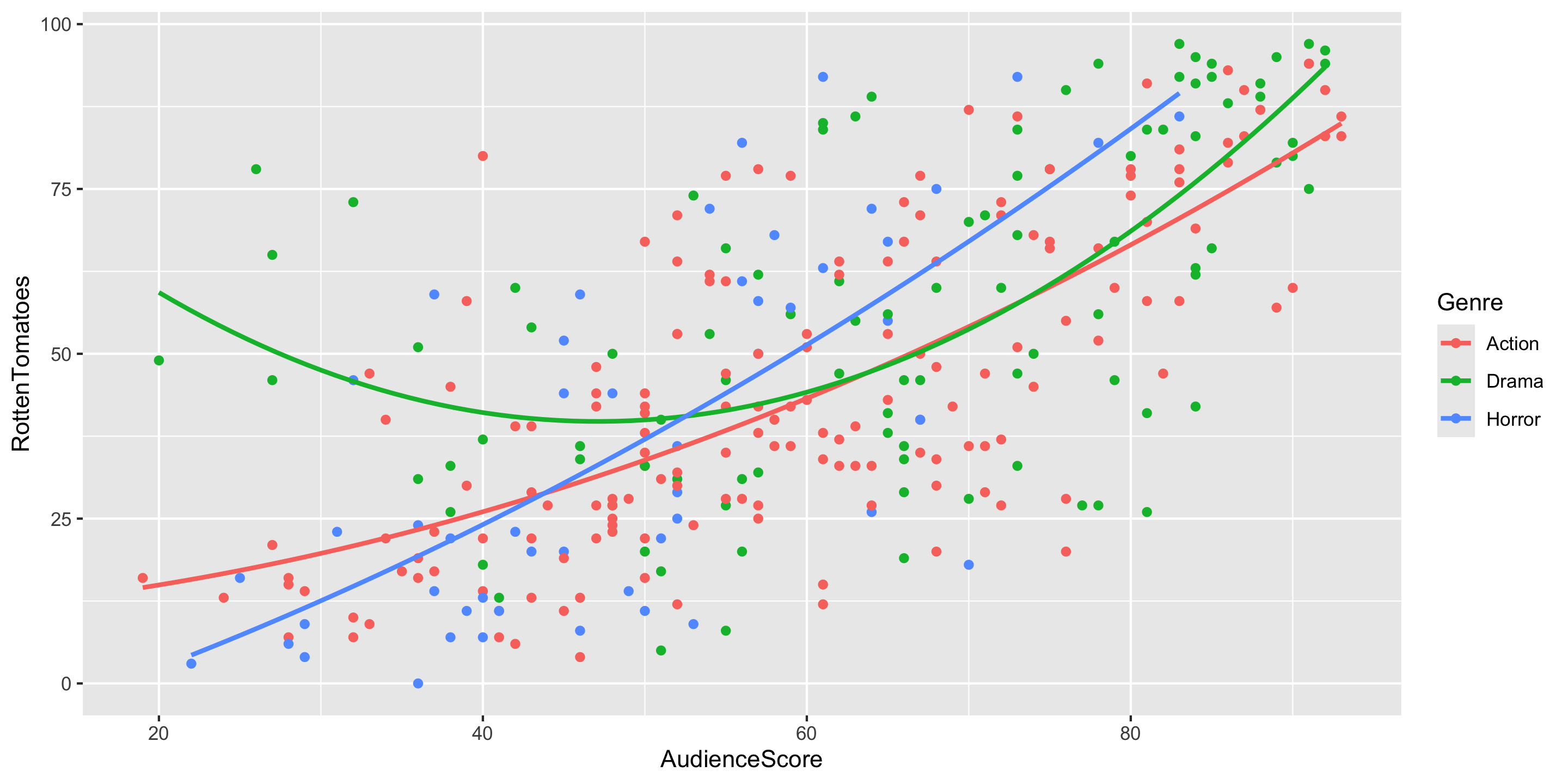
Adding a Curve to your Scatterplot
ggplot(data = movies2 %>% filter(Genre == "Drama"),
       mapping = aes(x = AudienceScore,
                     y = RottenTomatoes)) +
  geom_point(color = "#55B84F") +
  geom_smooth(method = "lm", se = FALSE, color = "#55B84F",
              formula = y ~ poly(x, degree = 2)) +
  ggtitle("Dramas Only") +
  theme(plot.title = element_text(size = 18))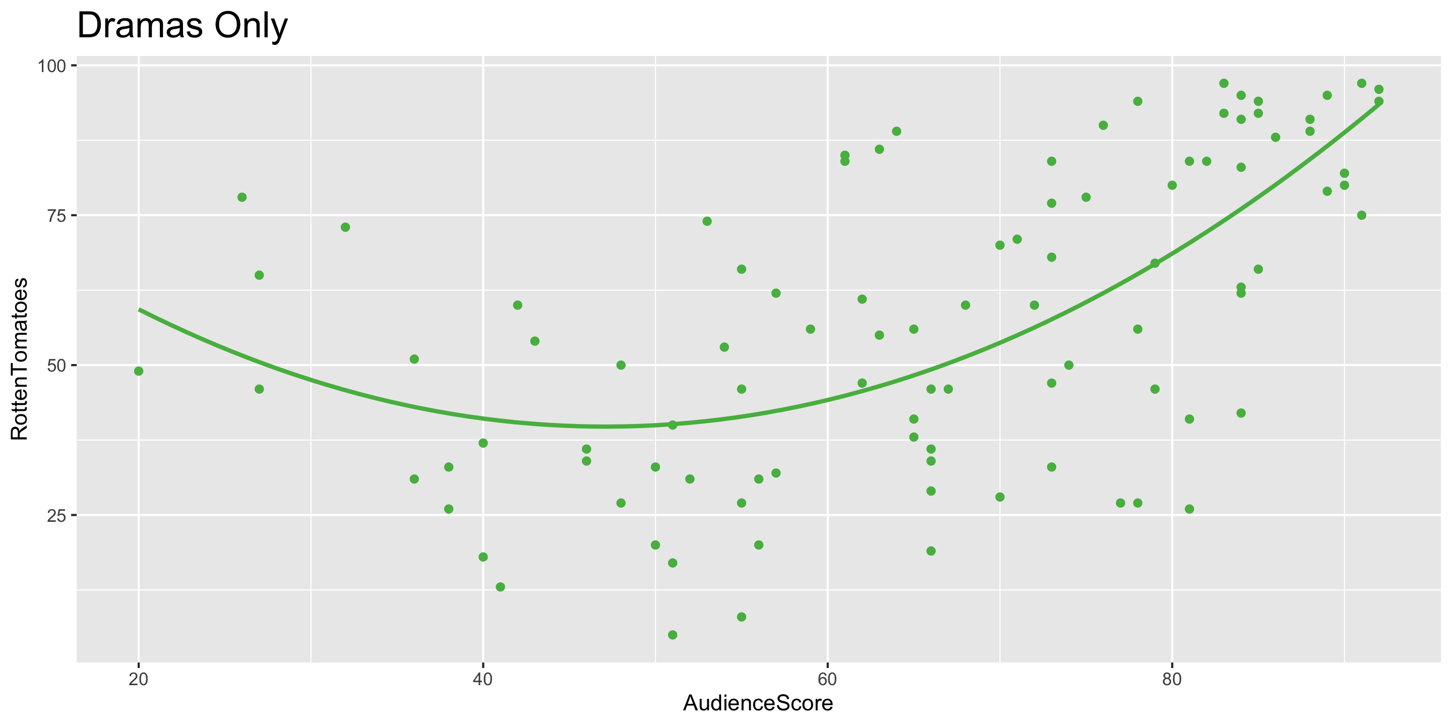
Using Transformations to Account for Non-Linear Relationships
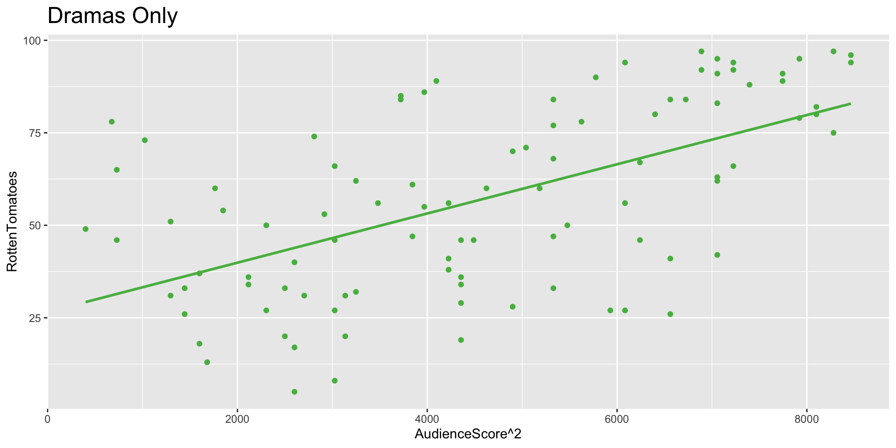
- Notice that the relationship between
AudienceScore\(^2\) andRottenTomatoesis approximately linear. AudienceScore\(^2\) is a transformation ofAudienceScore
Model Building Guidance
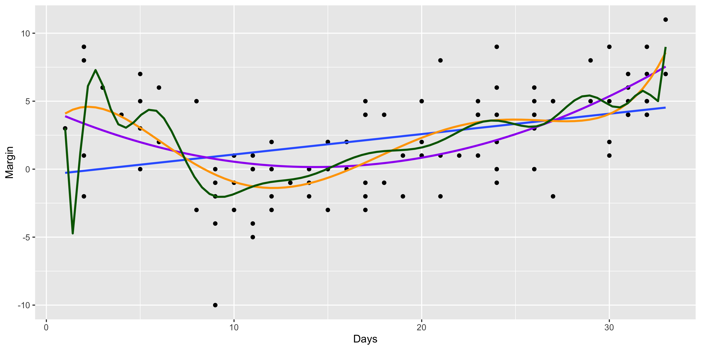
What degree of polynomial should I include in my model?
Guiding Principle: Capture the general trend, not the noise.
\[ \begin{align} y &= f(x) + \epsilon \\ y &= \mbox{TREND} + \mbox{NOISE} \end{align} \]
2008 Election Polls Example: