Linear Models III: Categorical Predictors
Megan Ayers
Math 141 | Spring 2026
Friday, Week 4
Exploratory Data Analysis
ggplot(candy, aes(x = factor(chocolate),
                   y = winpercent,
                  fill = factor(chocolate))) +
  geom_boxplot() +
  stat_summary(fun = mean,
               geom = "point",
               color = "yellow",
               size = 4) +
  guides(fill = "none") +
  scale_fill_manual(values =
                      c("0" = "deeppink",
                        "1" = "chocolate4")) +
  scale_x_discrete(labels = c("No", "Yes"),
                   name =
          "Does the candy contain chocolate?")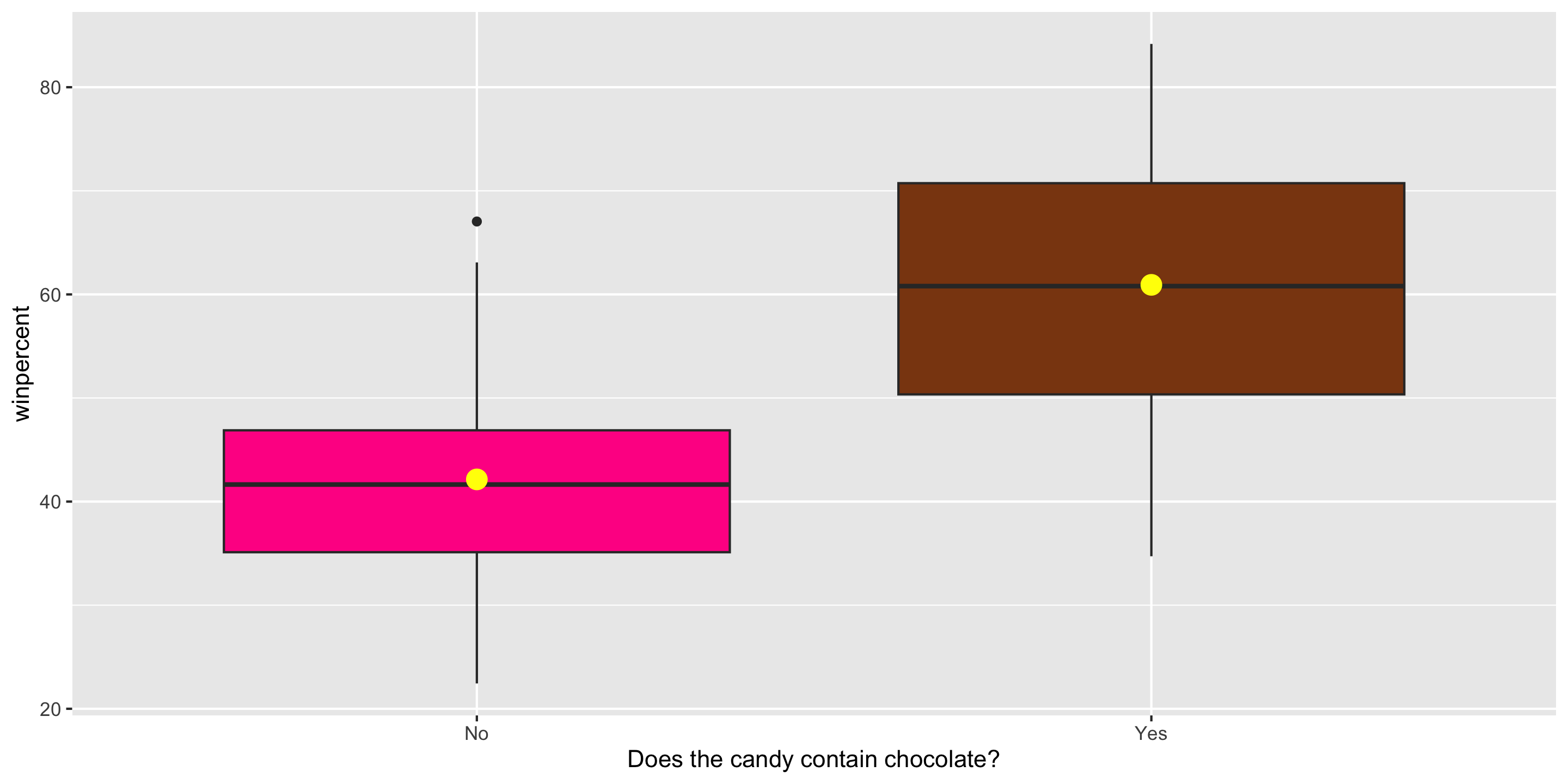
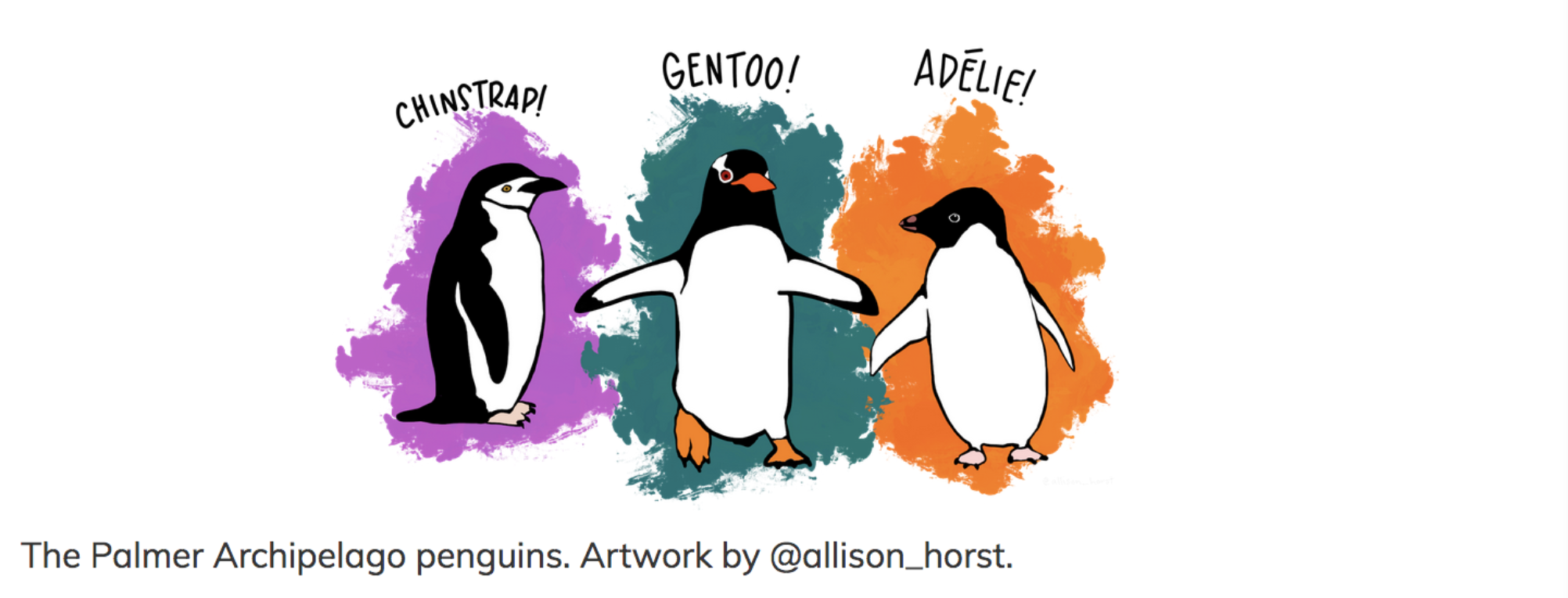
New example: Palmer Penguins
Exploratory data analysis
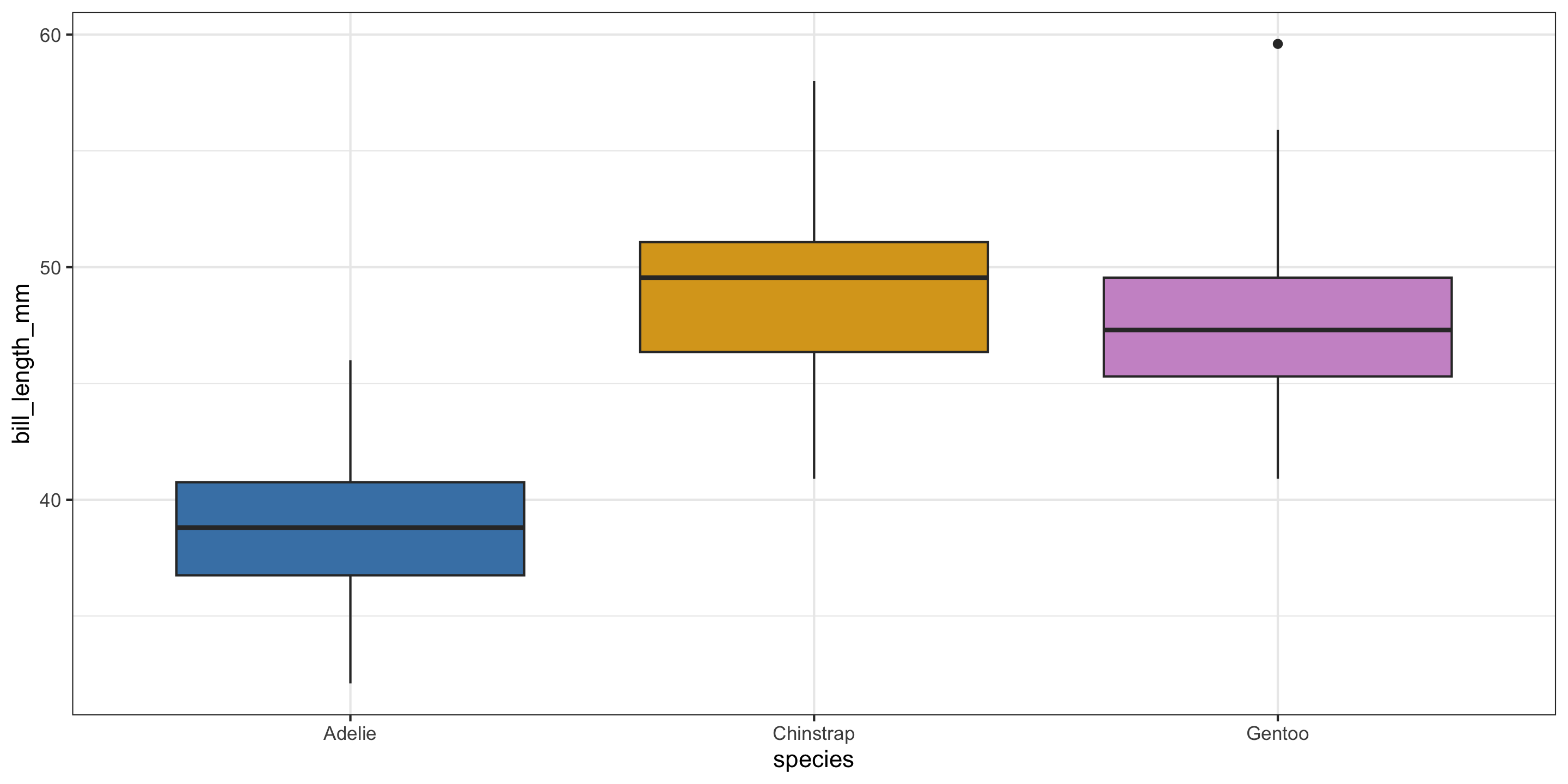
How do we handle more than 2 groups???