Note: A large slope does not necessarily indicate strong correlation, and a small slope does not necessarily indicate lack of correlation.
Method of Least Squares
Then we can estimate the whole function with:
\[
\widehat{y} = \widehat{\beta}_0 + \widehat{\beta}_1 x
\]
Called the least squares line, regression line, or the line of best fit.
Constructing the Simple Linear Regression Model in R
We can use the lm() function to construct the simple linear regression model in R and the get_regression_table() function from moderndive to interpret it.
mod <-lm(winpercent ~ sugarpercent, data = candy)get_regression_table(mod)
We need to be precise and careful when interpreting estimated coefficients!
Intercept: We expect/predict\(y\) to be \(\widehat{\beta}_0\)on average when \(x = 0\).
Slope: For a one-unit increase in \(x\), we expect/predict\(y\) to change by \(\widehat{\beta}_1\) units on average.
These interpretations are non-specific to the context of our model, but when we are interpreting coefficients, we always need to interpret the coefficients in context
We can always find the line of best fit to explore data, but…
To make accurate predictions or inferences, certain conditions should be met.
To responsibly use linear regression tools for prediction or inference, we require:
Linearity: The relationship between explanatory and response variables must be approximately linear
Check using scatterplot of data, or residual plot
Independence: The observations should be independent of one another.
Can check by considering data context, and
sometimes by looking at scatterplots/residual plots
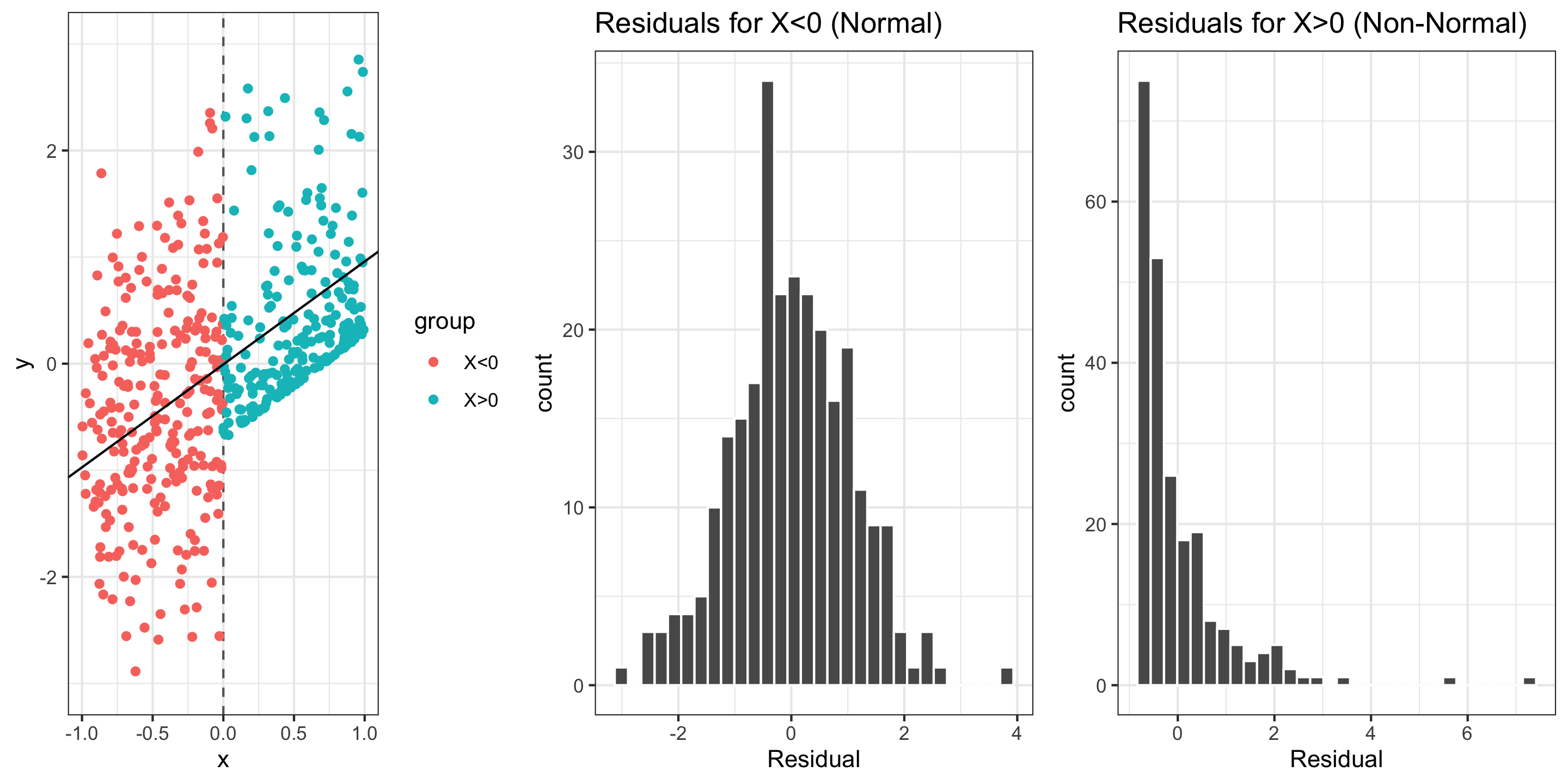
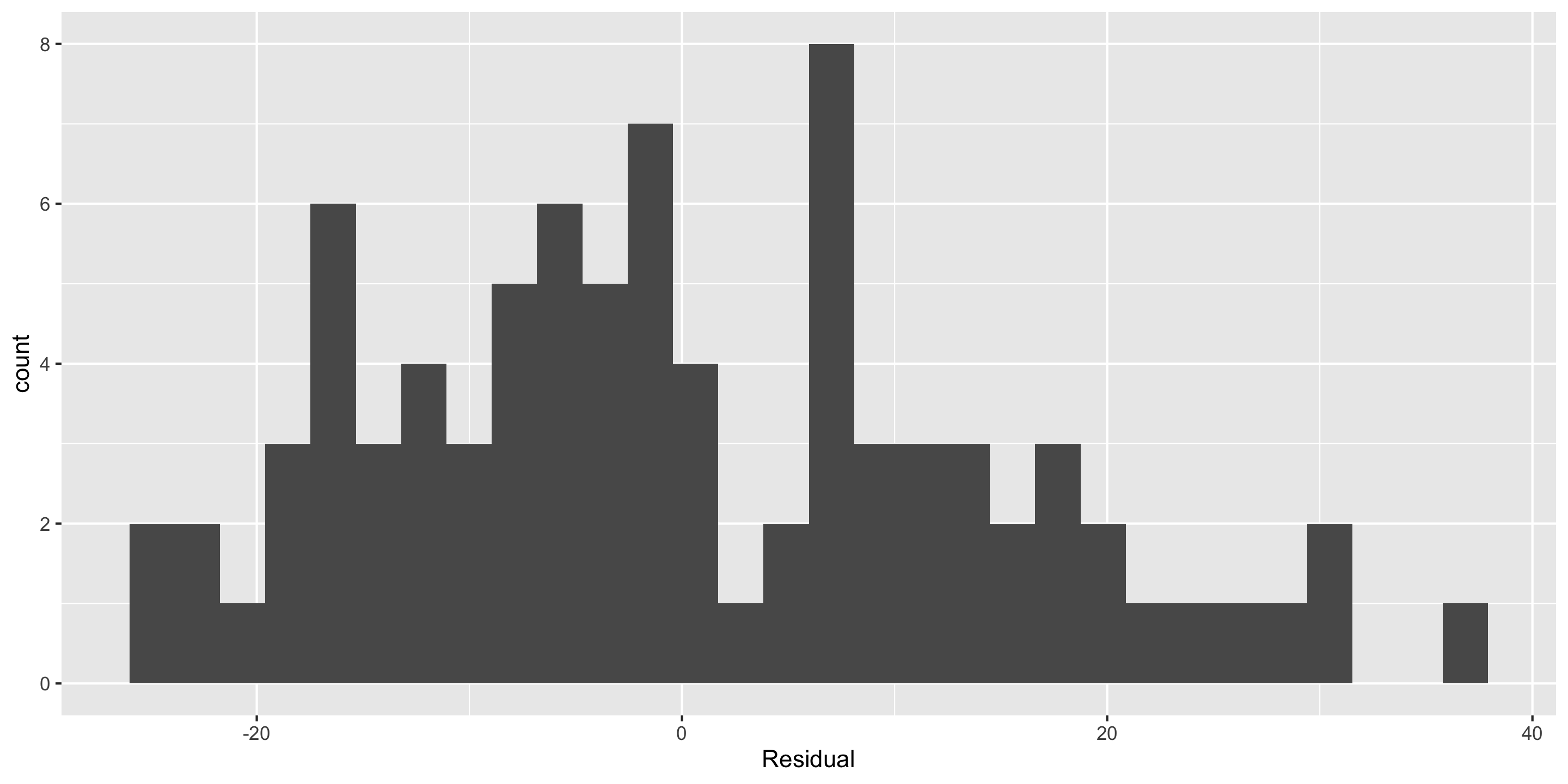
Normality: The distribution of residuals should be approximately bell-shaped, unimodal, symmetric, and centered at 0 at every “slice” of the explanatory variable
Simple check: look at histogram of residuals
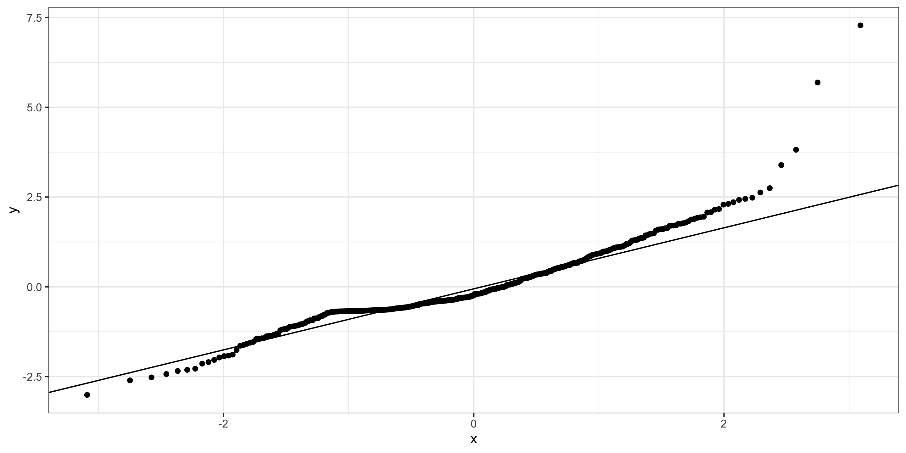
Better to use a Q-Q plot
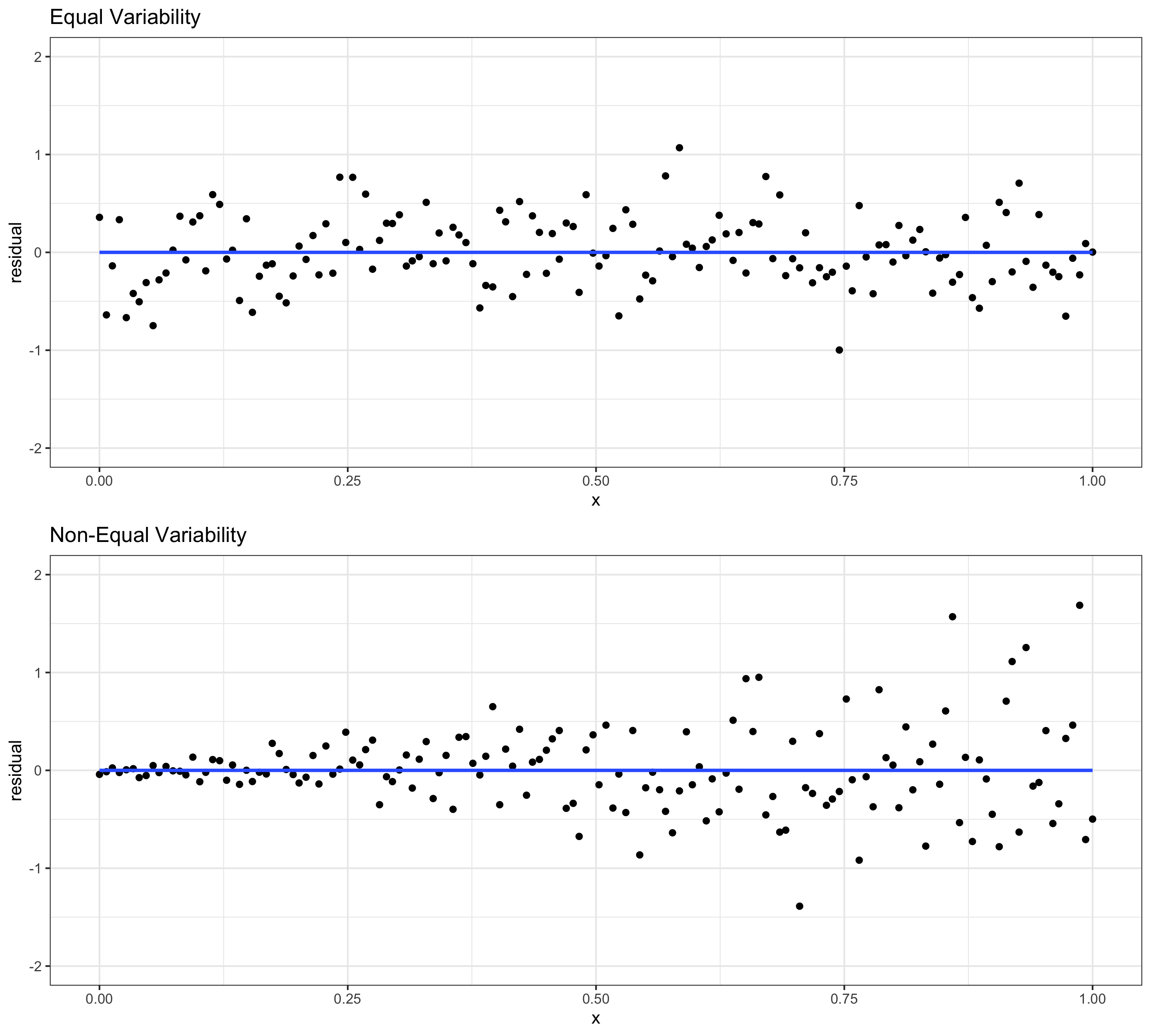
Equal Variability: Variance of residuals should be roughly constant across data set. Also called “homoscedasticity”. Models that violate this assumption are sometimes called “heteroscedastic”
Check using residual plot.
A cute way to remember this: “LINE”
Linearity
Independence
Normality
Equal Variability
We assess these using diagnostic plots (y vs x scatterplot, residual plot, residual histogram, q-q plot)
Later in the course, we’ll learn why I, N, and E are required for inference
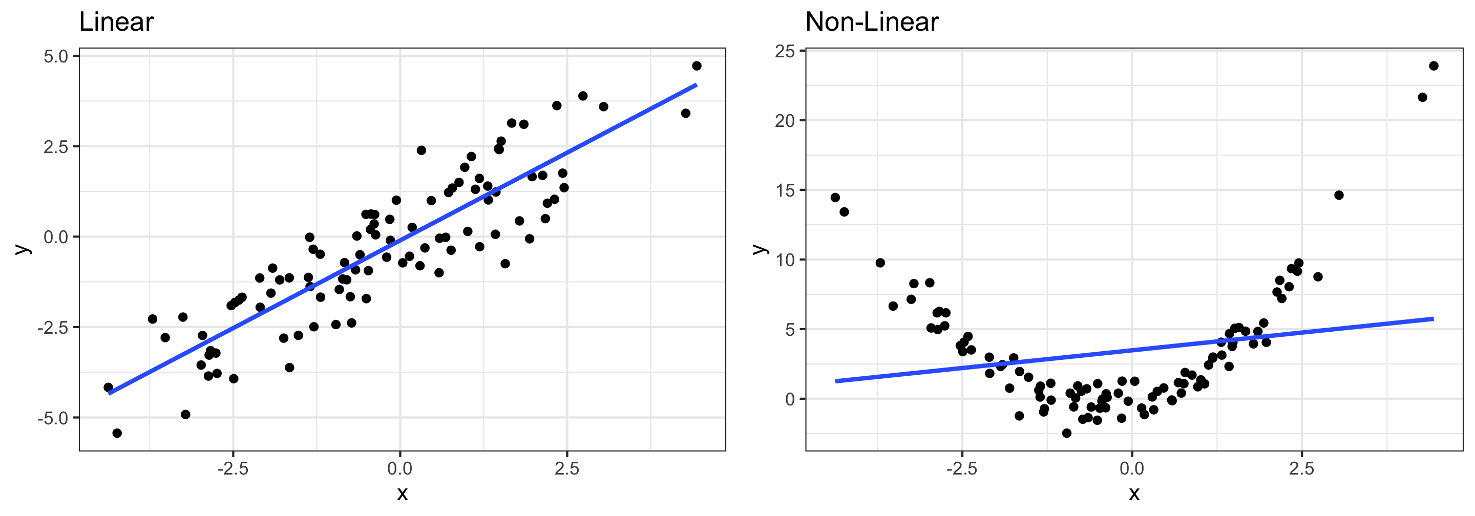
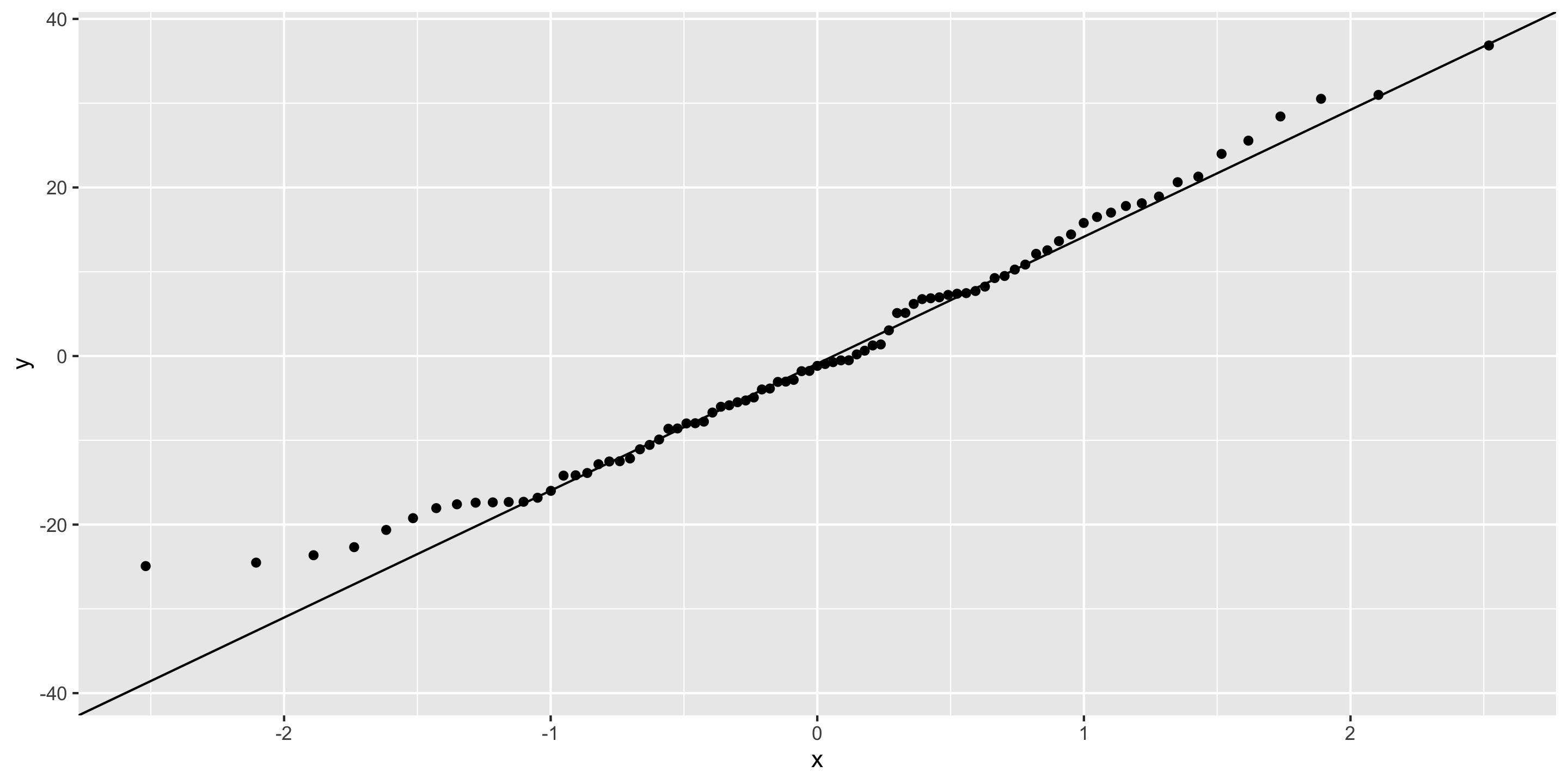
Assessing conditions: Linearity
Linearity: The relationship between explanatory and response variables must be approximately linear
Points should be evenly distributed above and below the regression line at each “slice” of x
If data is non-linear:
Slope does not adequately describe relationship and predictions can be very inaccurate
More advanced modeling techniques should be used instead (take STAT 243)
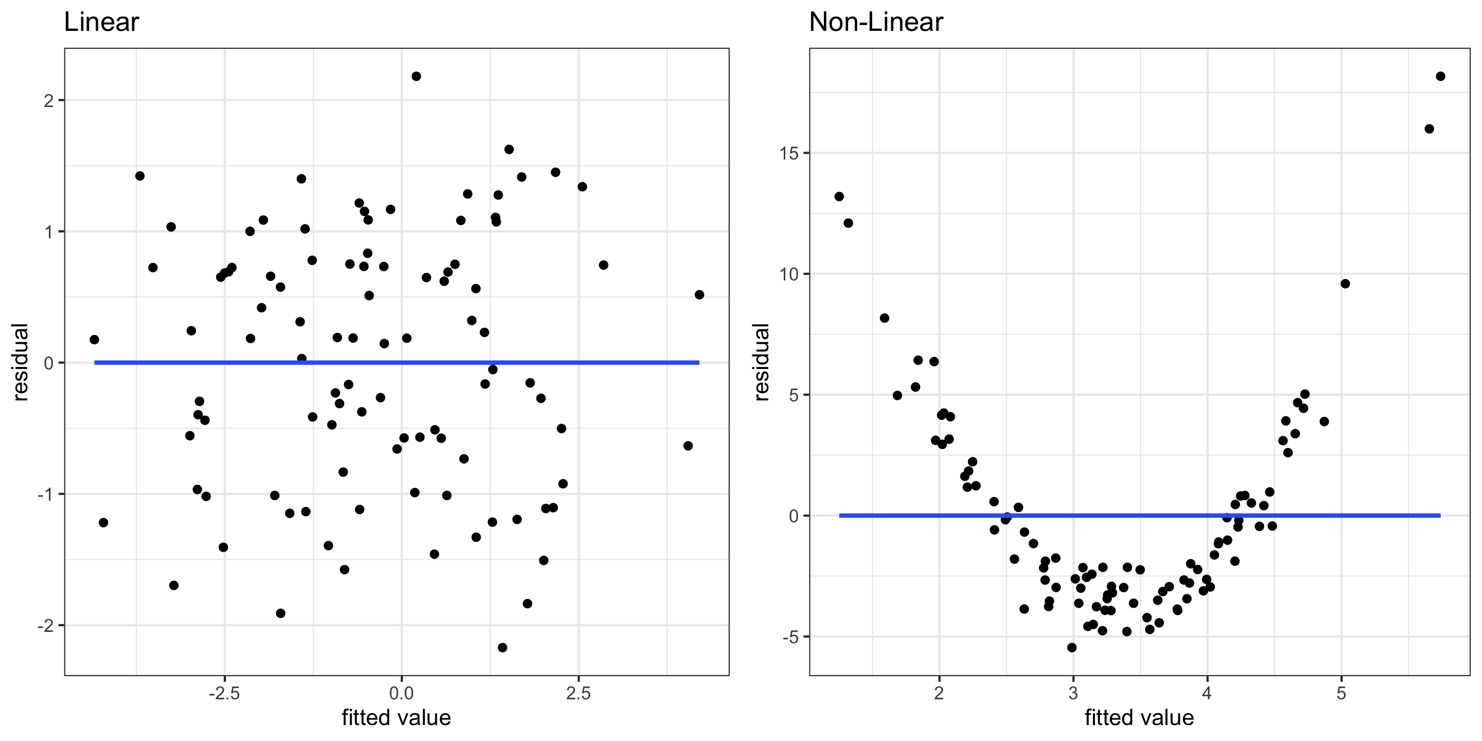
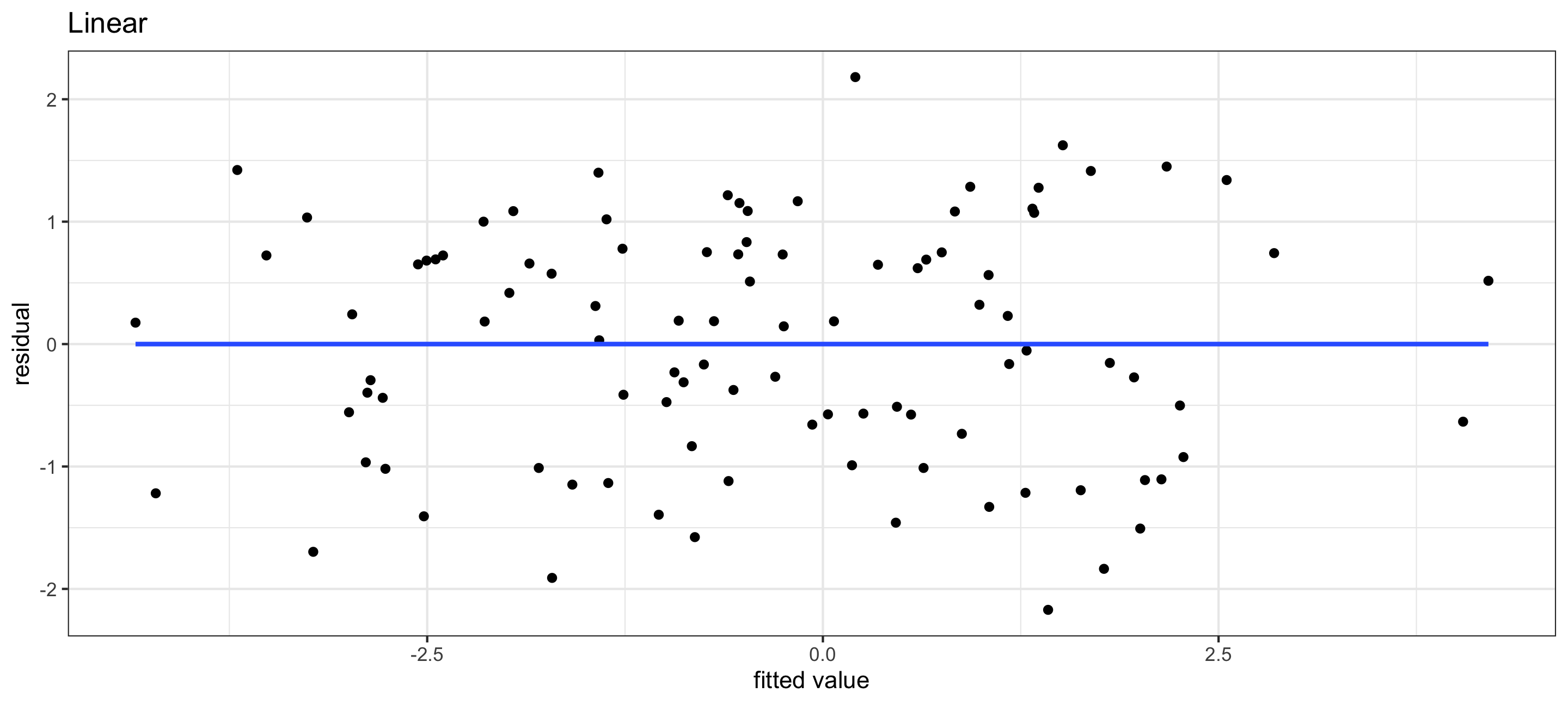
Assessing conditions: Linearity
Residual plots can also be useful for checking linearity
These plot model residuals against the fitted values
We don’t want to see any trends here
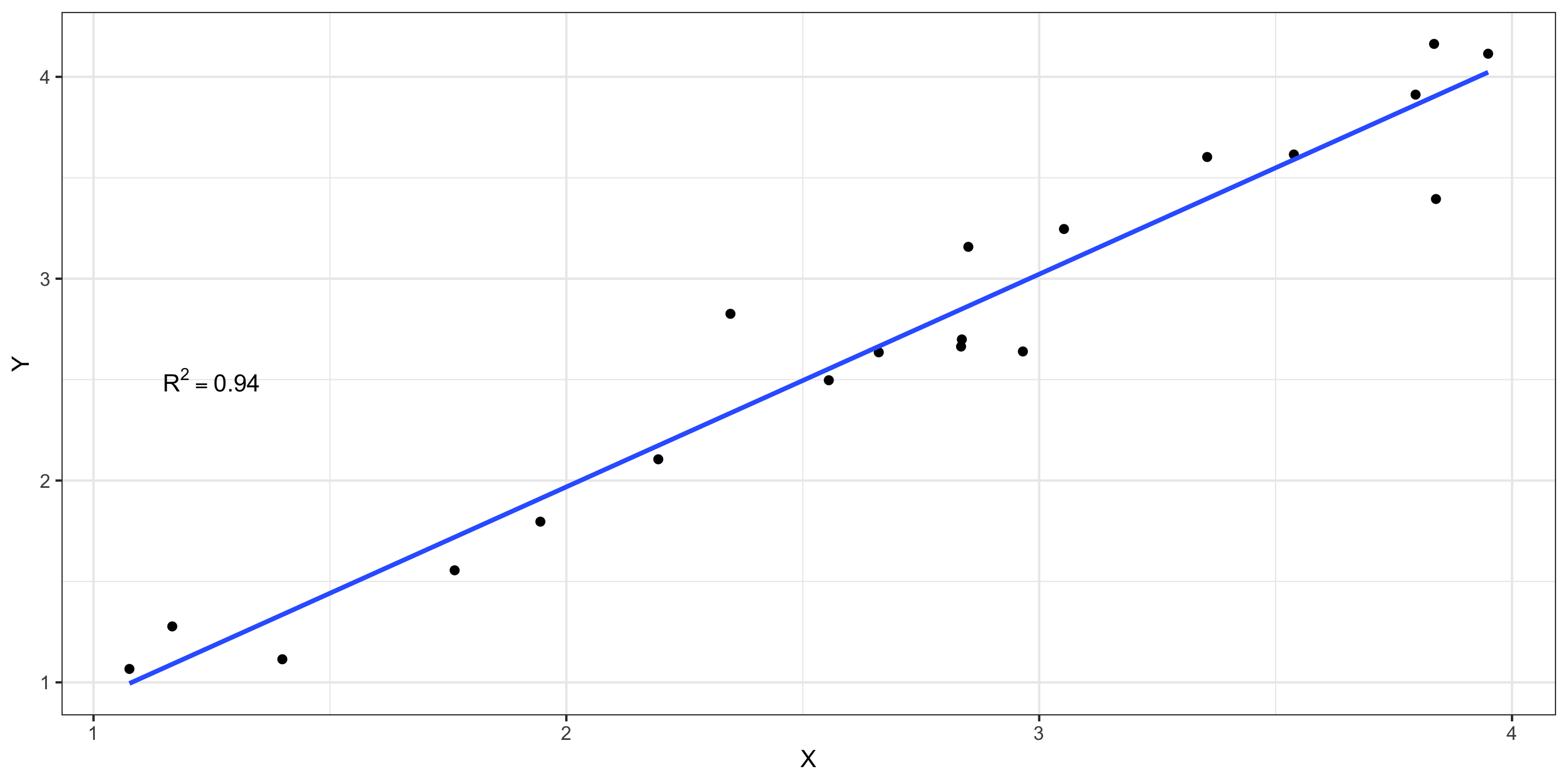
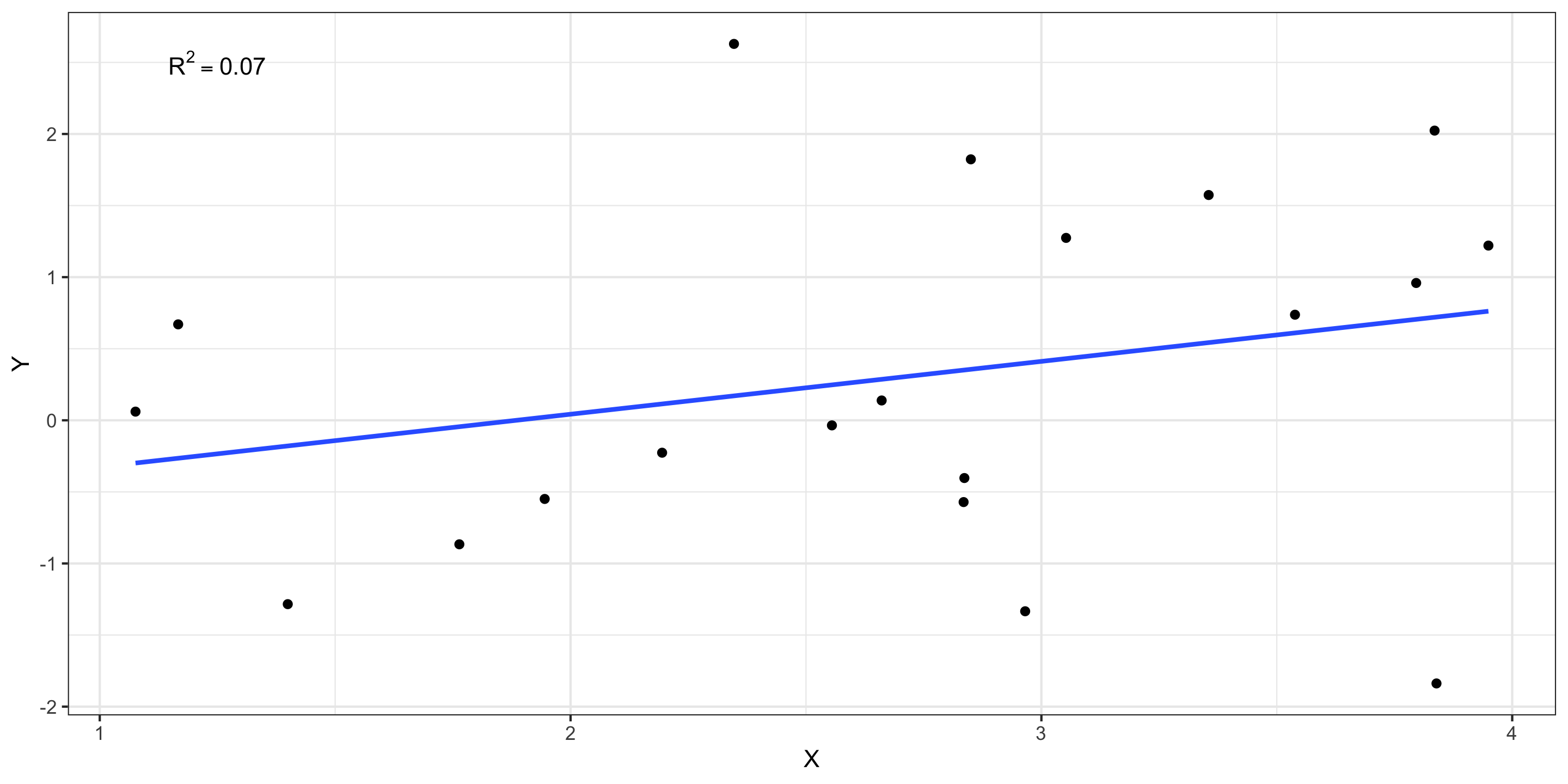
Assessing conditions: Linearity (Code Example)
library(moderndive)# Creating the modellm1 <-lm(data = my_df, y1 ~ x)# *** Pulling out model inputs, residuals, and fitted values ***res1 <-get_regression_points(lm1) # Plotting residuals vs fitted values(g1 <-ggplot(res1, aes(x = y1_hat, y = residual)) +geom_point() +theme_bw() +geom_smooth(method ="lm", se = F) +labs(x ="fitted value", y ="residual", title ="Linear"))
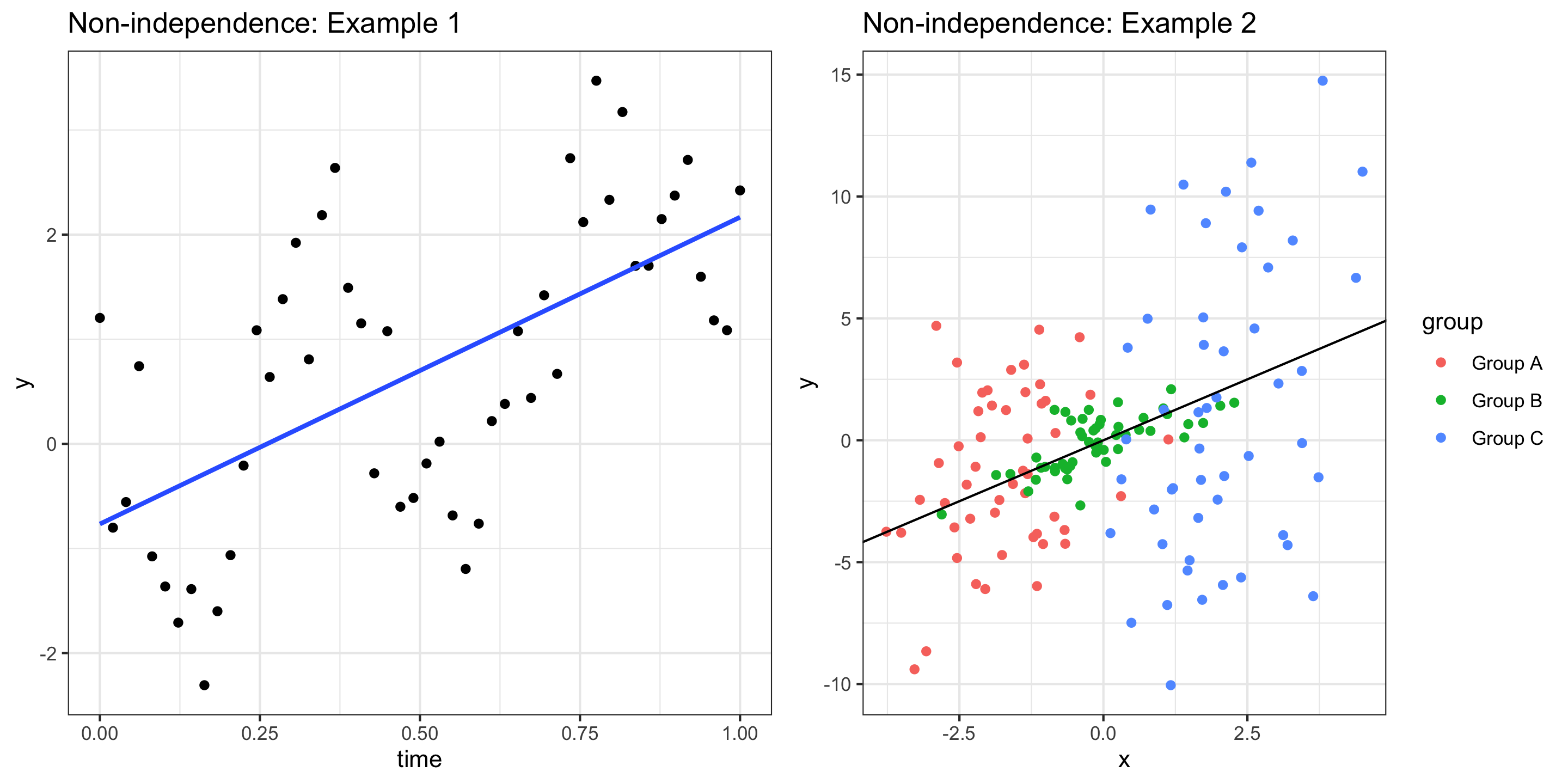
Assessing conditions: Independence
Independence: The observations should be independent of one another
If observations are not independent, inference about the population may be misleading.
We usually assess independence qualitatively
Are observations inherently connected? (Beyond variables in the model)
Assessing conditions: Normality (of residuals)
Normality: The distribution of residuals should be bell-shaped, unimodal, symmetric, and centered at 0 at every “slice” of the explanatory variable
Assessing conditions: Normality (of residuals)
Normality: The distribution of residuals should be bell-shaped, unimodal, symmetric, and centered at 0 at every “slice” of the explanatory variable
If residuals are non-Normal…
Some predictions can be very inaccurate
Inference about the population may be misleading
Assessing conditions: Normality (of residuals)
Normality: The distribution of residuals should be “Normal”
Equal Variability: Variance of residuals should be approximately constant across the data
Residual plots are also very useful for this
If equal variability isn’t met:
Inference about the population may be misleading
(Potential) outliers in high-variability range are more influential
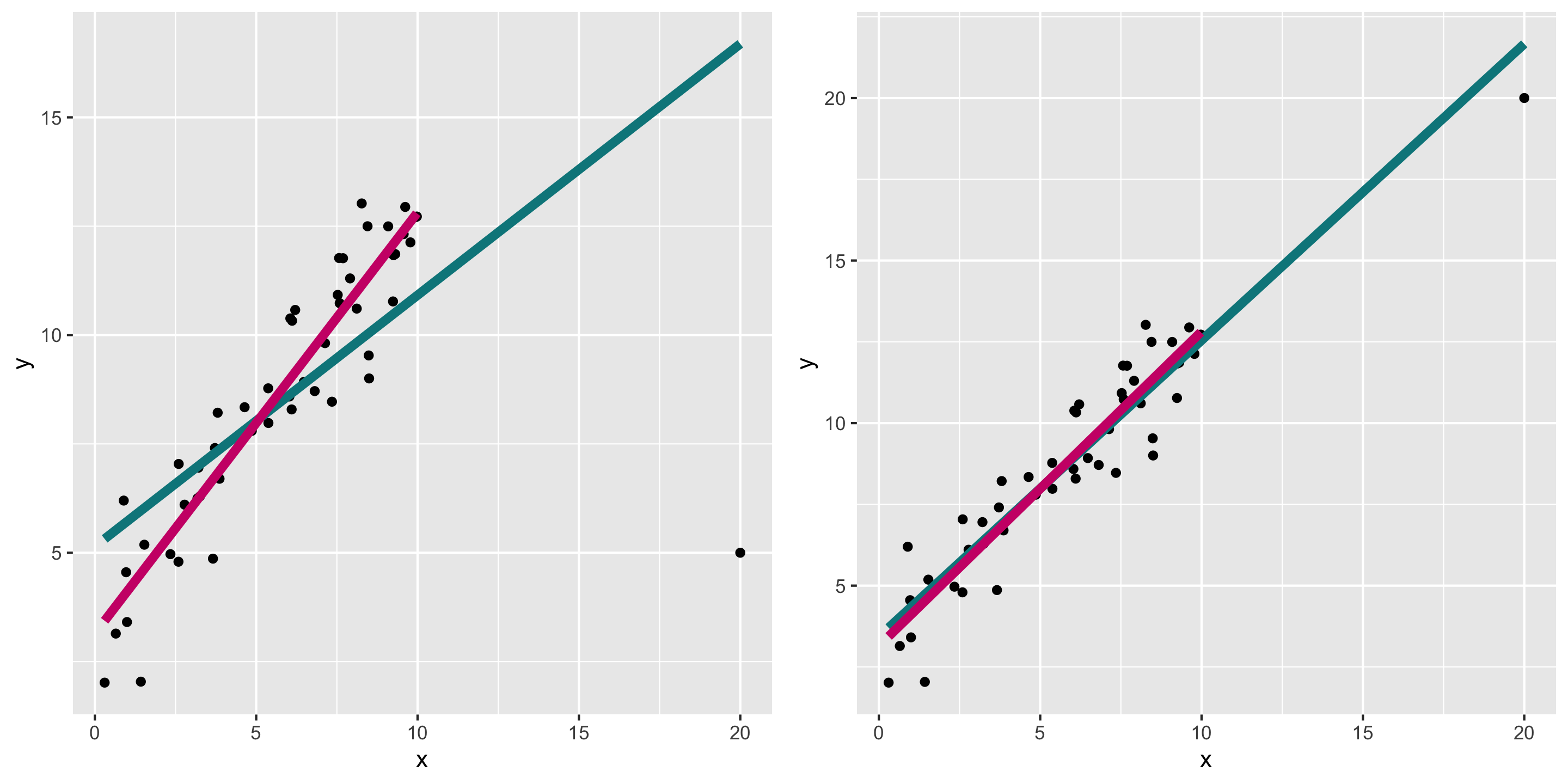
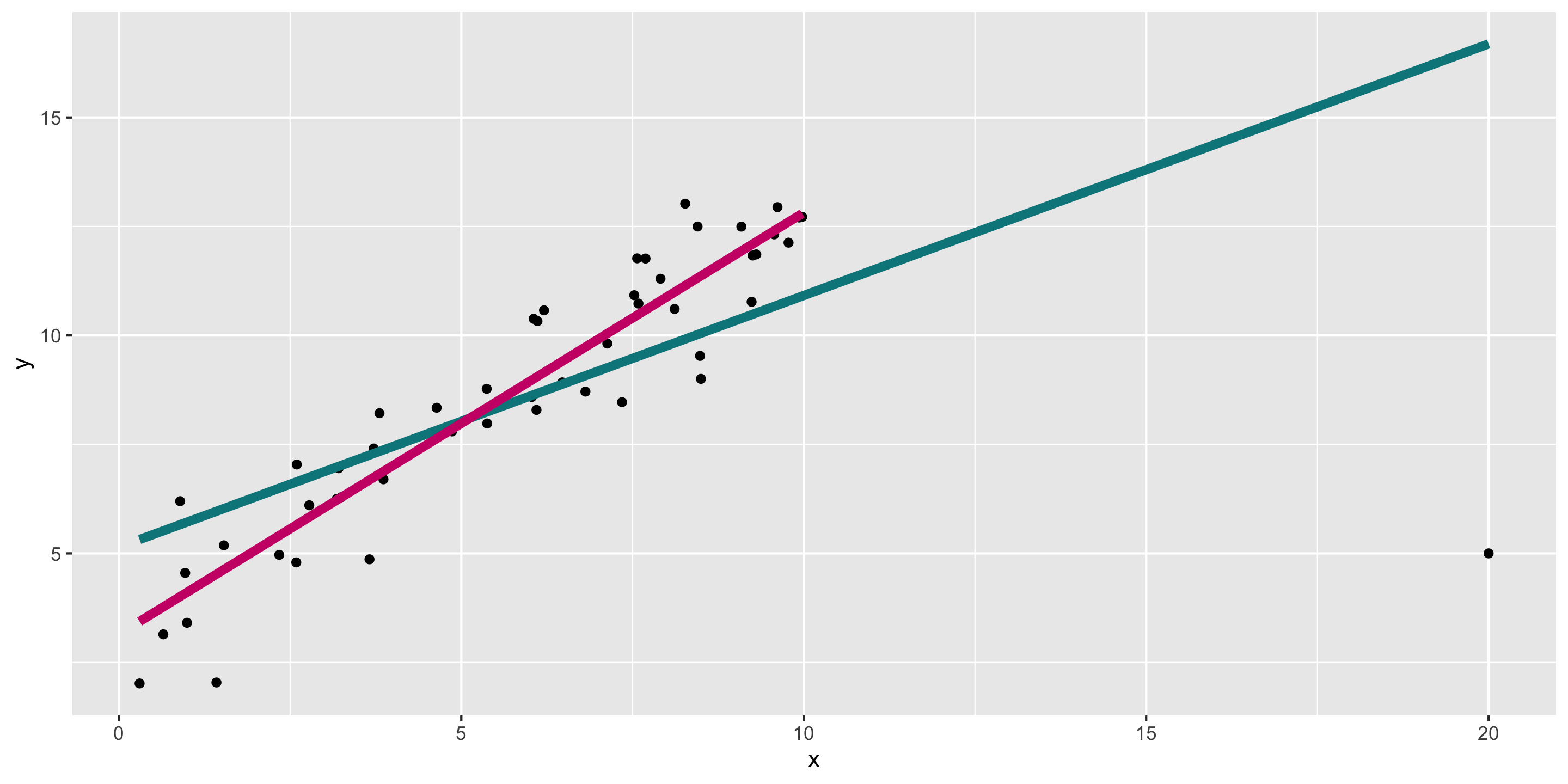
Another example: high leverage points
Remember the outlier example:
What do diagnostics look like when we fit the teal model?
Diagnosing the model
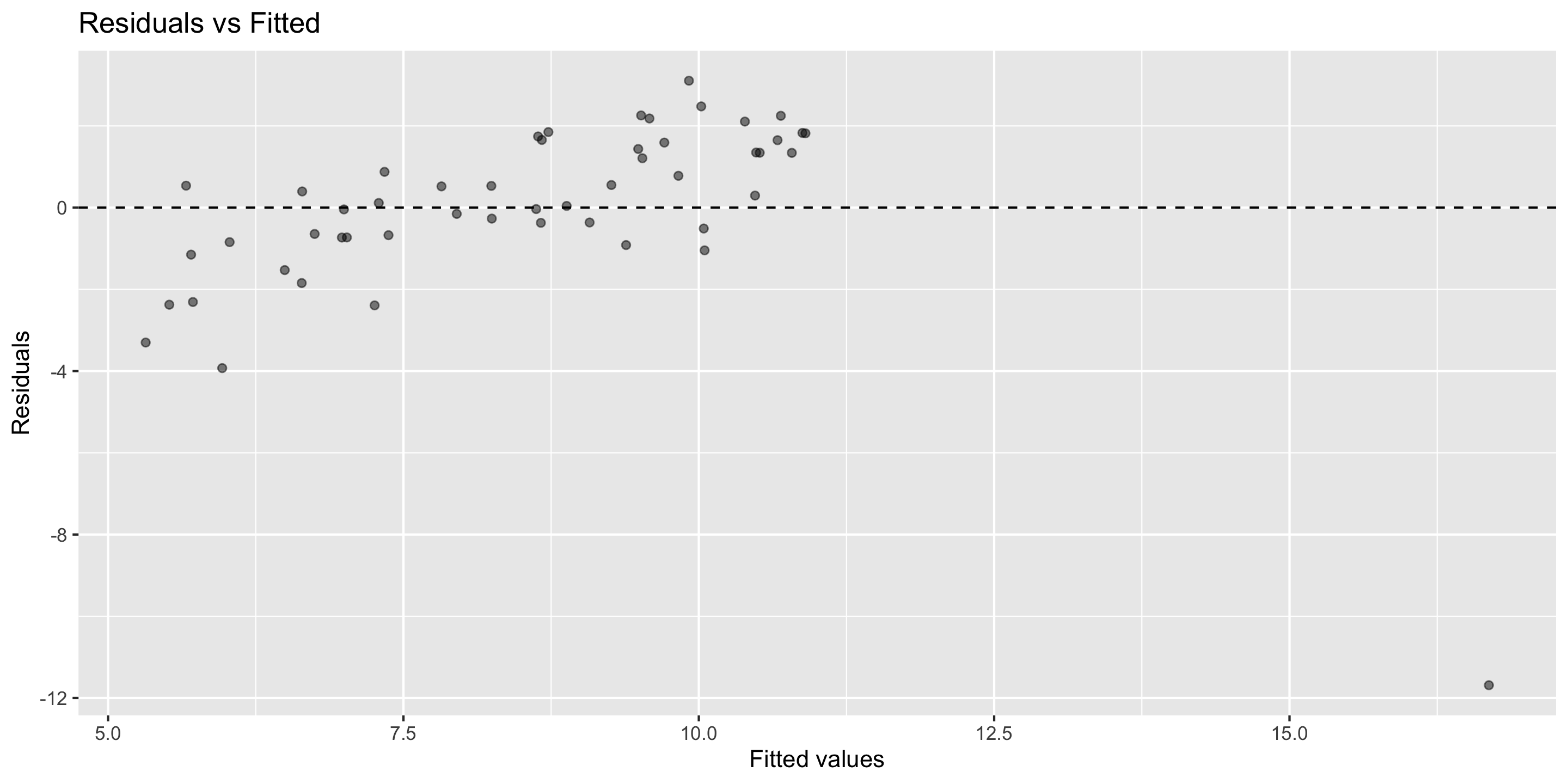
In this case, can already see the outlier in the residual vs fitted plot.
What to do with high leverage points?
Depends on context
It may be reasonable to remove them and refit the model
If we believe the data is the result of an error
If we are most focused on prediction for non-outliers, or if our population of interest does not include the outlier
But we shouldn’t remove outliers just because we don’t like the results that they produce
Especially if our goal is descriptive or explanatory, and the outlier represents a valid data point
dat_no_outlier <- dat %>%filter(x <15)pink_mod <-lm(y ~ x, dat_no_outlier)
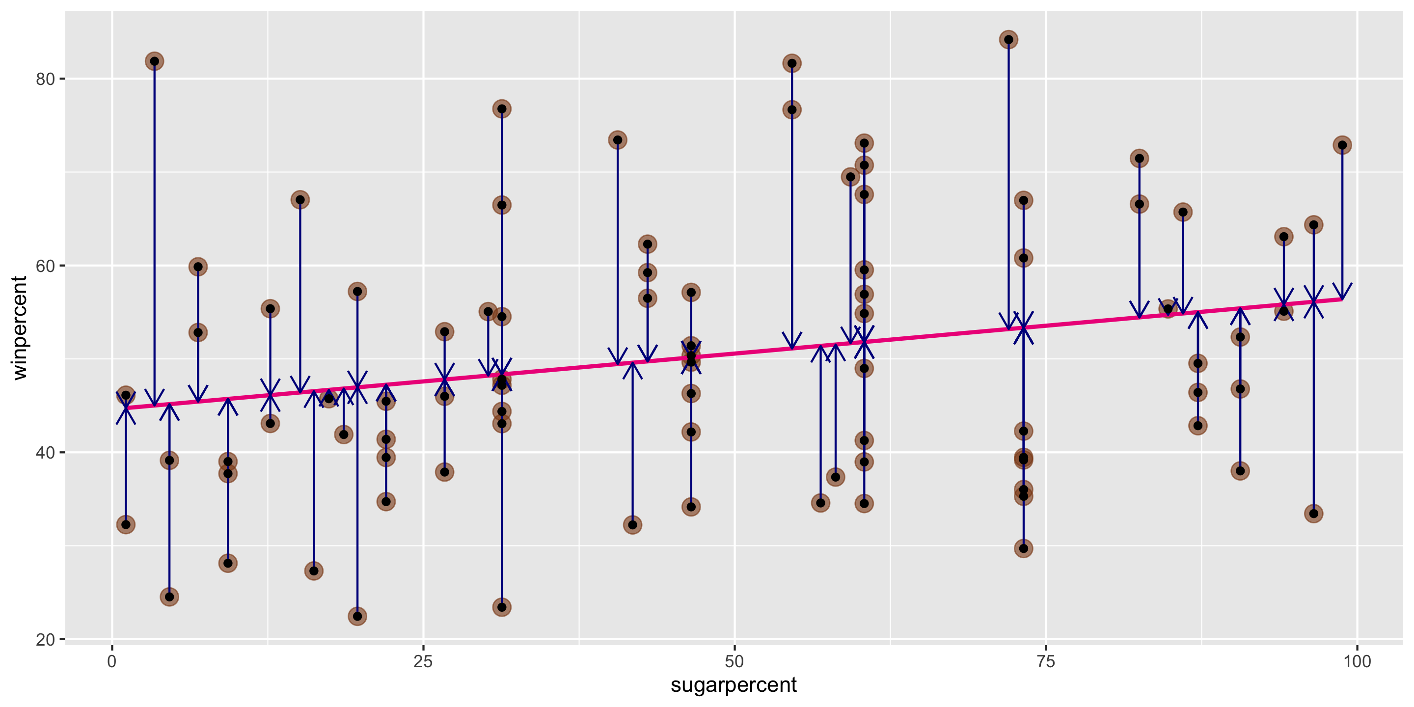
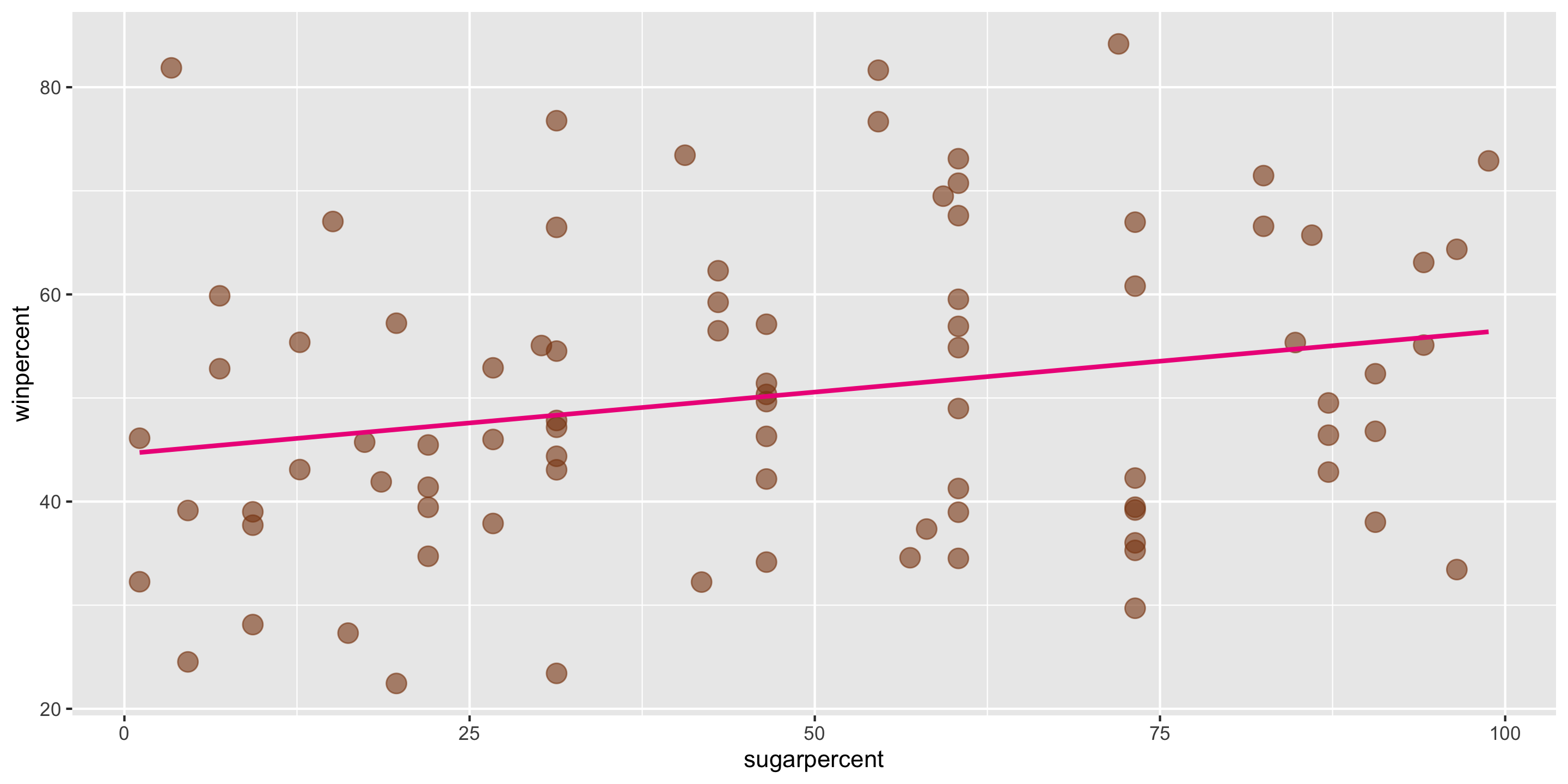
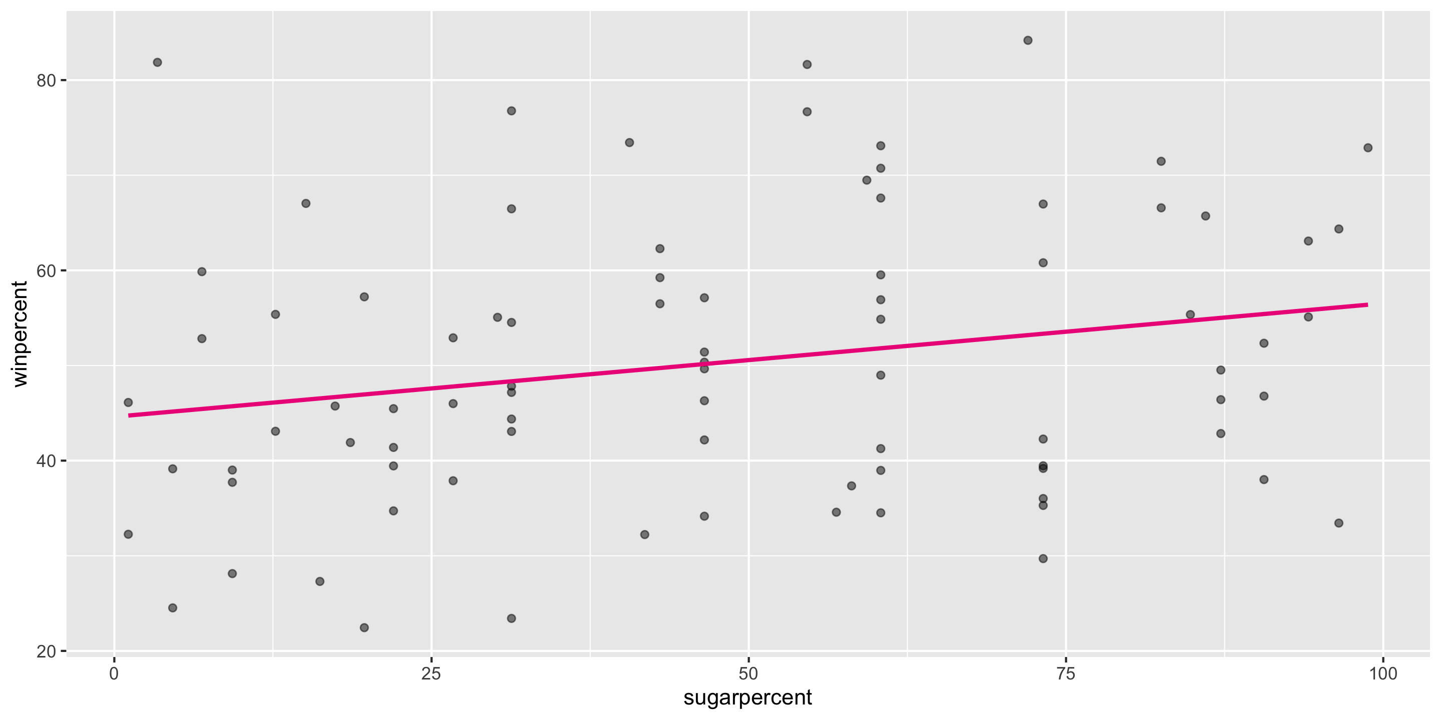
Recall our candy simple linear regression model
mod <-lm(winpercent ~ sugarpercent, data = candy)
Let’s check if this meets the LINE assumptions
Q: First, what does this graph tell us about Linearity?
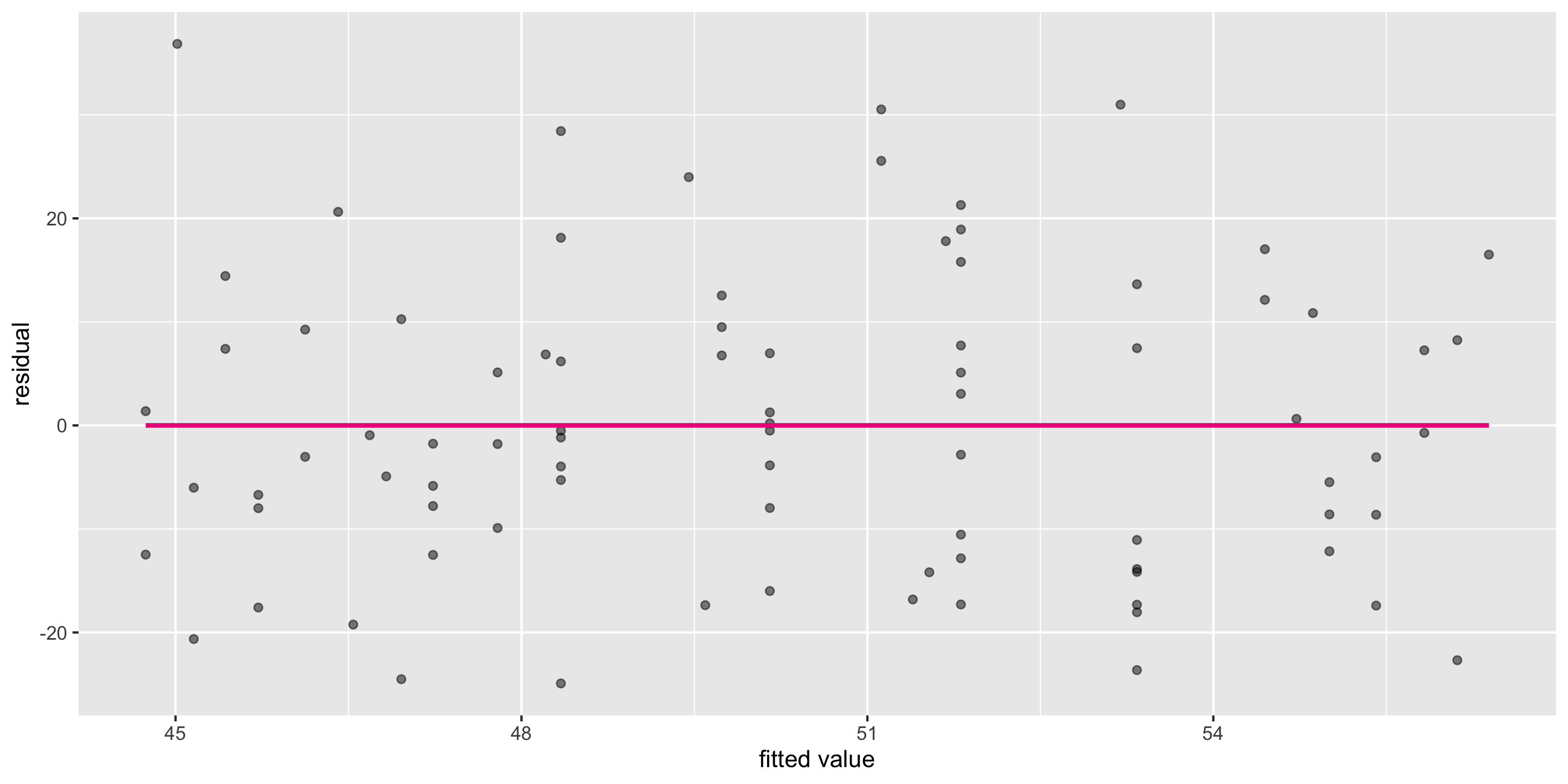
Residual vs. fitted plot
res <-get_regression_points(mod)ggplot(res, aes(x = winpercent_hat, y = residual)) +geom_point(alpha =0.5) +geom_smooth(method ="lm", se =FALSE, color ="deeppink2") +labs(x ="fitted value", y ="residual")