

Linear Models I: Introduction
Megan Ayers
Math 141 | Spring 2026
Monday, Week 4
Example: The Ultimate Halloween Candy Power Ranking
Linear trend?
Direction of trend?
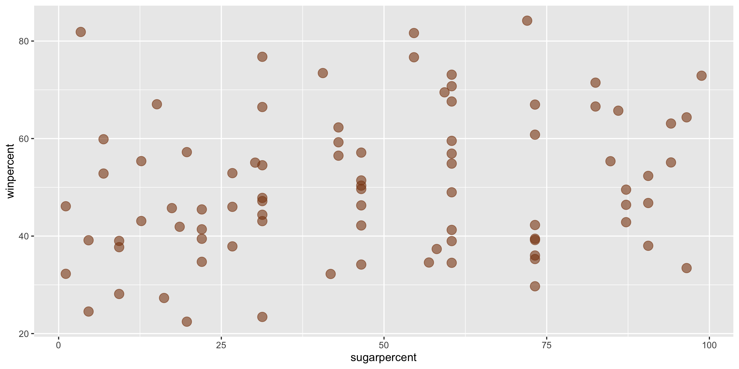
Example: The Ultimate Halloween Candy Power Ranking
- A simple linear regression model would be suitable for these data:
\[ y = \beta_0 + \beta_1 x + \epsilon \]
- \(\beta_0\) and \(\beta_1\) are fixed numbers
- \(\beta_0\) represents the intercept of a line
- \(\beta_1\) represents the slope of a line

- Knowing \(\beta_0\) and \(\beta_1\) would help us summarize and describe the relationship between \(x\) and \(y\).
We want to find \(\beta_1\) (slope) and \(\beta_0\) (intercept) so that the line fits our data well
→ Need summary statistics that quantify the strength and relationship of the linear trend
→ These will help us find a value for slope and determine how well a line fits our data
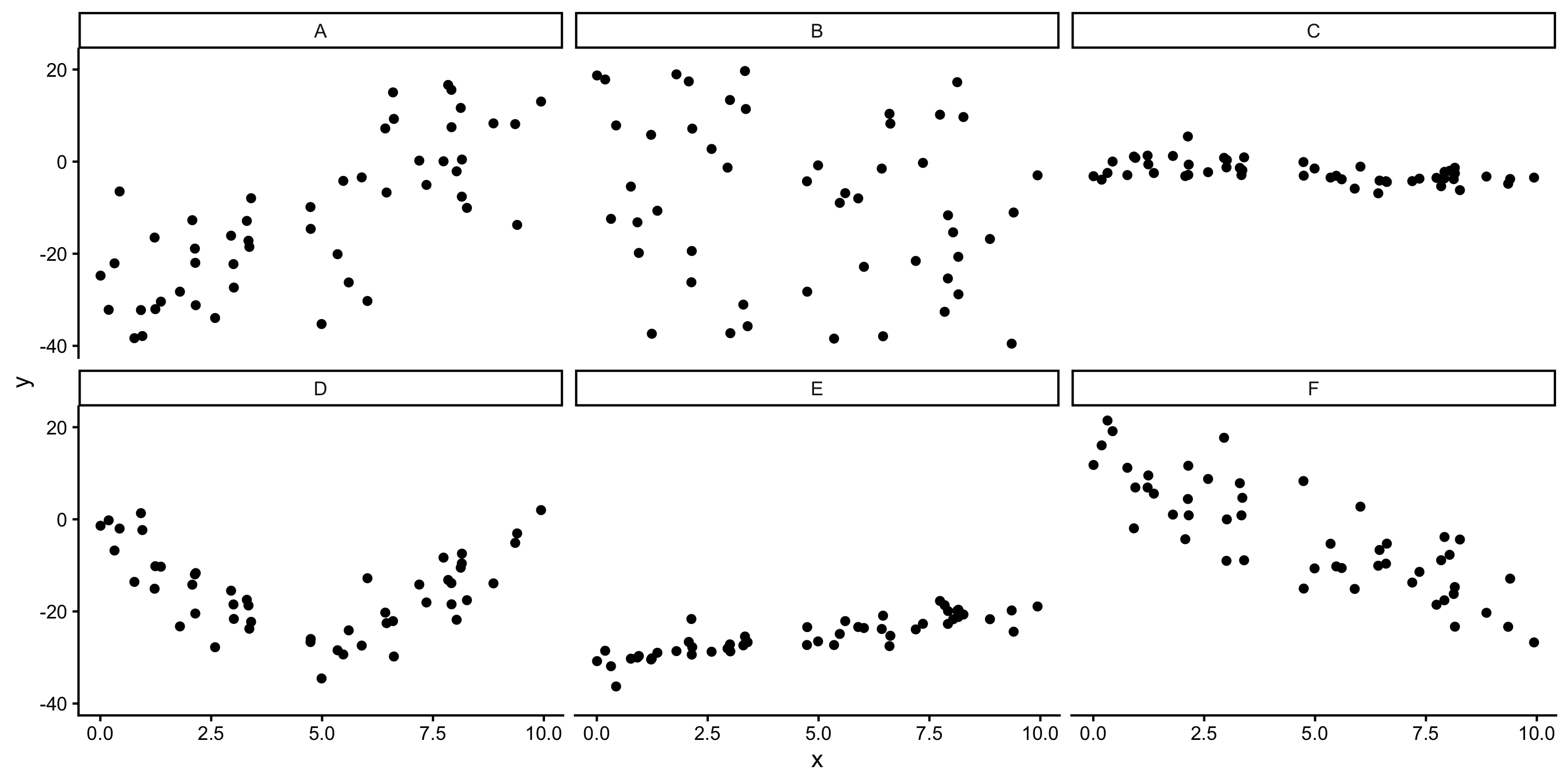
Correlation, Covariance, and Slope
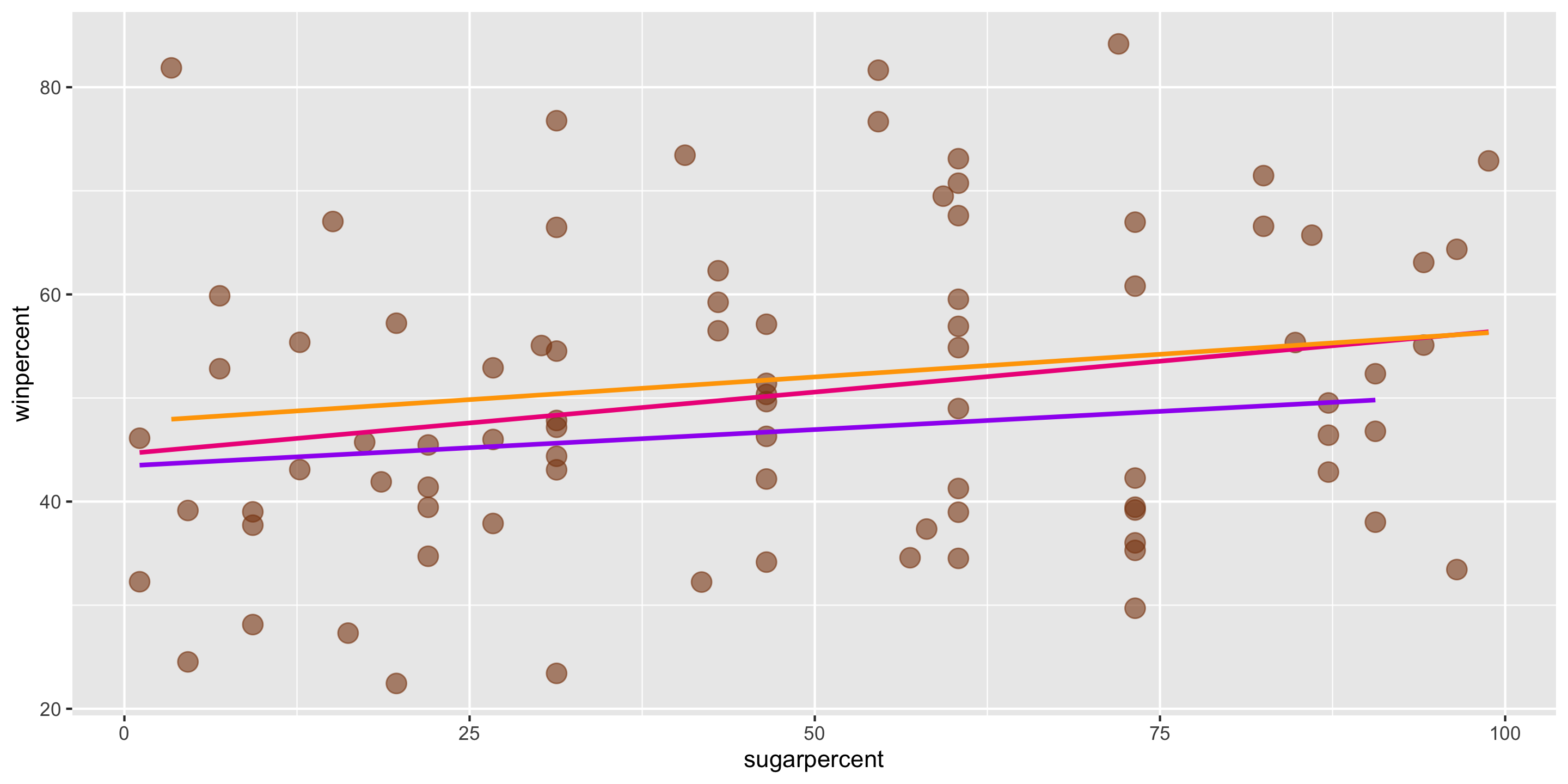
Q: Which will have the largest positive correlation?
Q: Which will have the largest negative correlation?
Q: Which will have correlation closest to 0?
A: 0.7568 B: -0.2172 C: -0.5373 D: -0.1133 E: 0.863 F: -0.8343 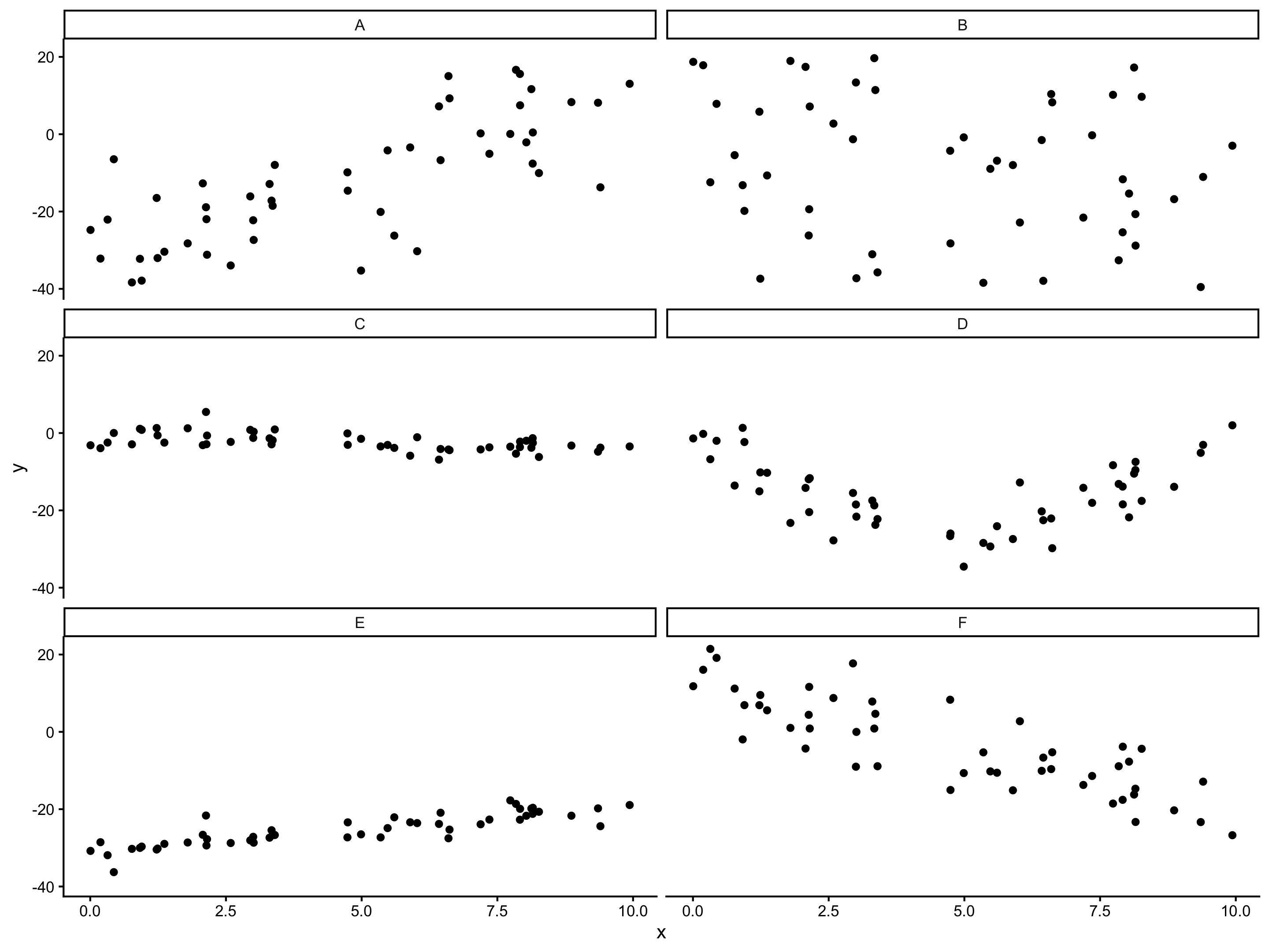
- Correlation: how strong is the linear relationship relative to noise
- Correlation and slope are related, but not the same (ex. A vs E)
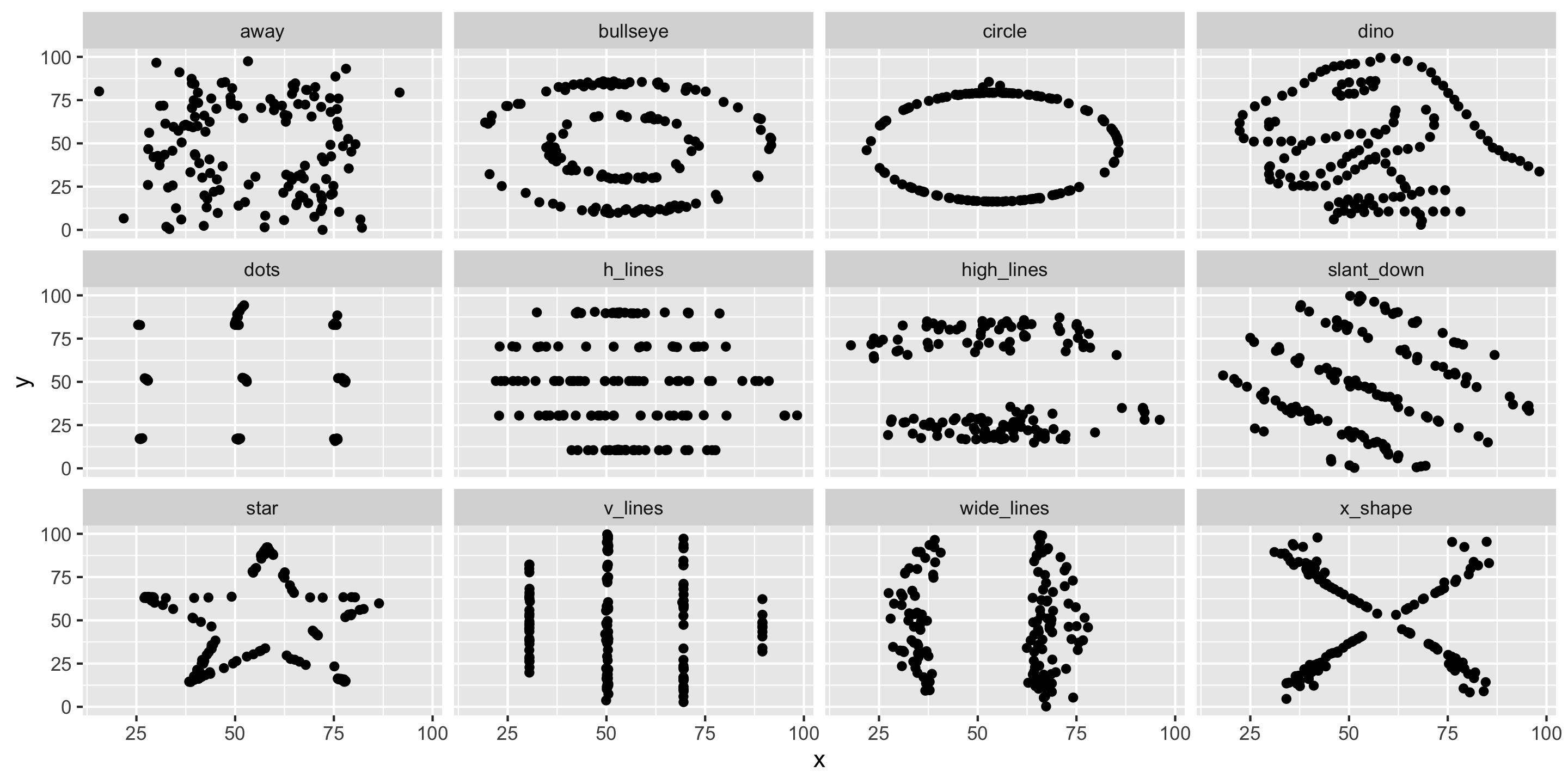
Always graph the data when exploring relationships!
Simple Linear Regression
Let’s return to the Candy Example.
A line is a reasonable model form.
Where should the line be?
- Slope? Intercept?
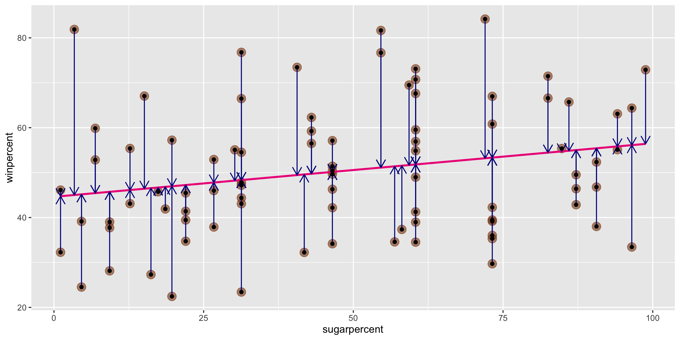
Method of Least Squares
Want residuals to be small.
Minimize a function of the residuals.
Minimize:
\[ \sum_{i = 1}^n e^2_i \]
Sidenote:
- We could use \(\sum_{i = 1}^n |e_i|\)
- But, this is less common, less computationally efficient, and lacks theoretical advantages
- \(\sum_{i = 1}^n e_i^2\) appropriately weights one large residual as “worse” than many small ones
Method of Least Squares
ggplot2 will compute the line and add it to your plot using geom_smooth(method = "lm")
We can calculate the exact values of \(\widehat{\beta}_0\) and \(\widehat{\beta}_1\) using our formulas, by hand or in R
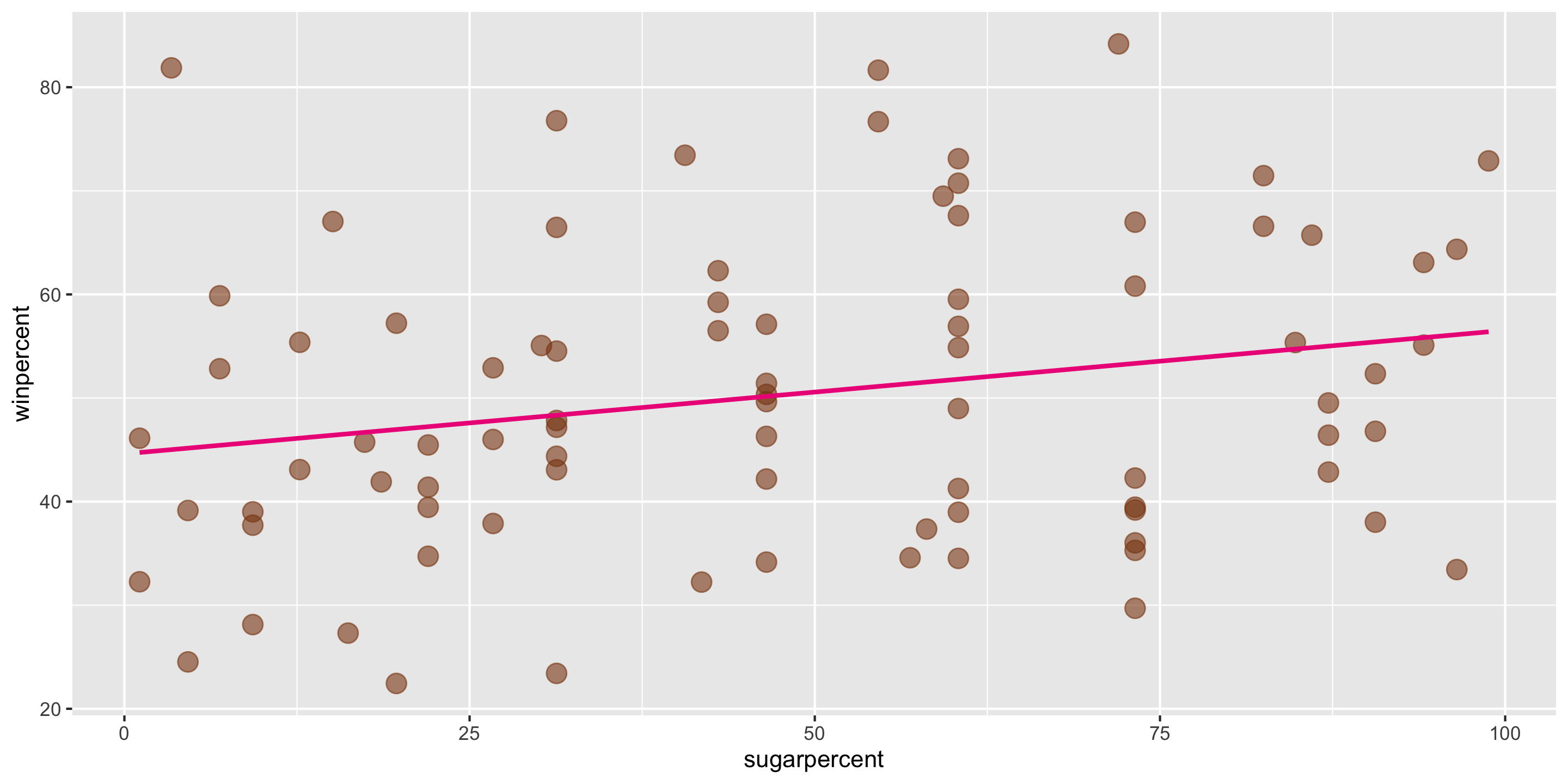
Method of Least Squares
\[ \widehat{y} = \widehat{\beta}_0 + \widehat{\beta}_1 x \] In this case, \(\widehat{\beta}_0 = 44.6094\) and \(\widehat{\beta}_1 = 0.1192\).

Method of Least Squares
\[ \widehat{y} = \widehat{\beta}_0 + \widehat{\beta}_1 x \] In this case, \(\widehat{\beta}_0 = 44.6094\) and \(\widehat{\beta}_1 = 0.1192\).
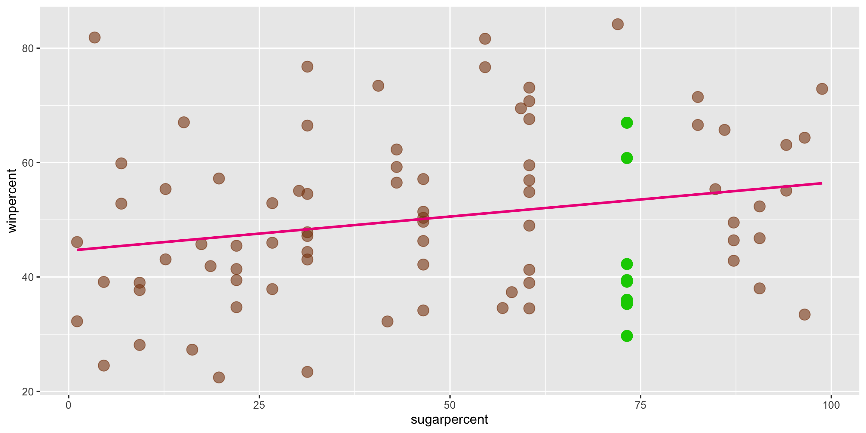
- Q: Suppose a new candy bar has
sugarpercent = 73. What does the model predict forwinpercent?
Method of Least Squares
\[ \widehat{y} = \widehat{\beta}_0 + \widehat{\beta}_1 x \] In this case, \(\widehat{\beta}_0 = 44.6094\) and \(\widehat{\beta}_1 = 0.1192\).
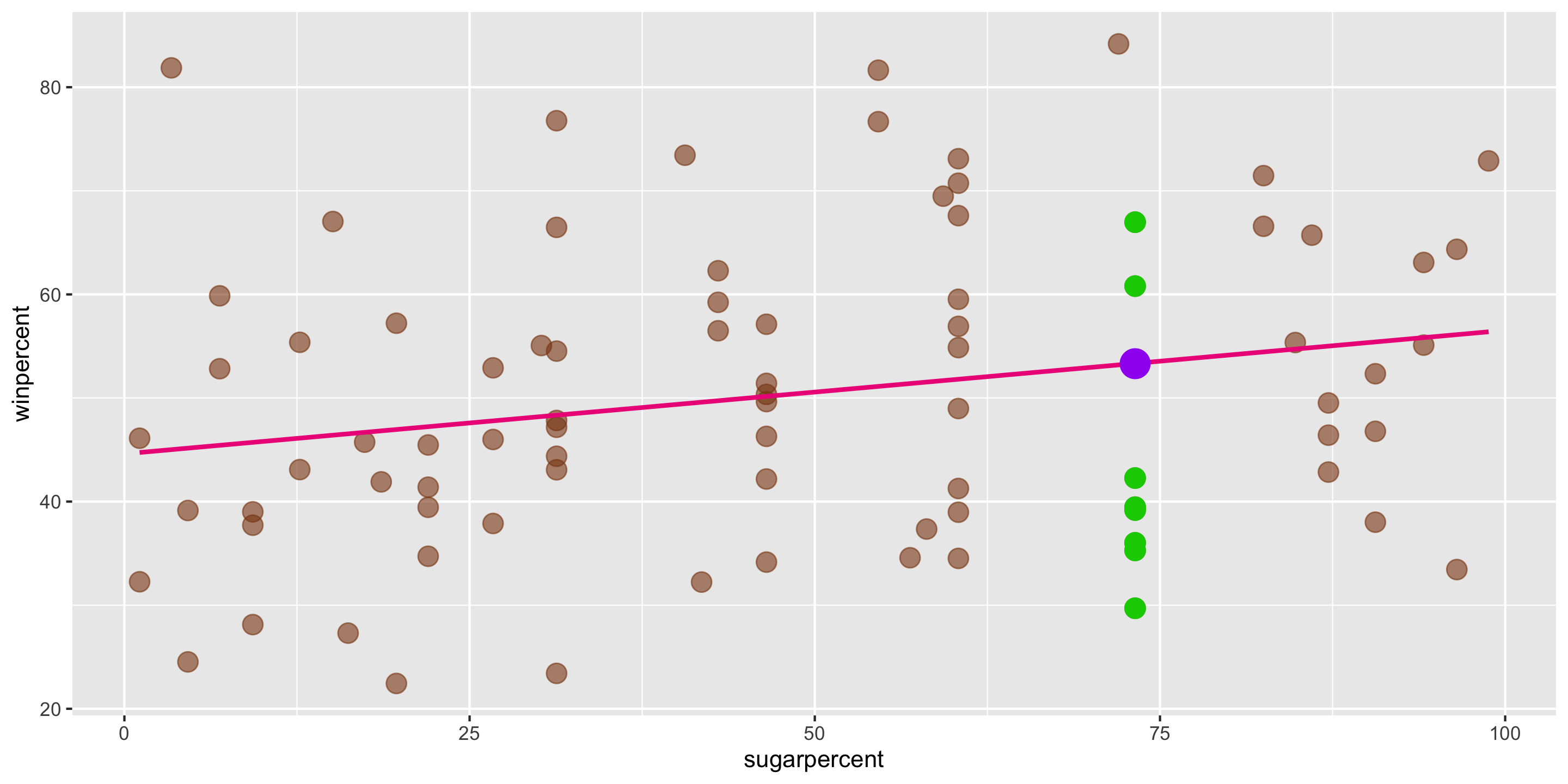
- Q: Suppose a new candy bar has
sugarpercent = 73. What does the model predict forwinpercent? - A: \(\widehat{y} = 44.6094 + 0.1192 \cdot 73\) = 53.311
- This is different from the actual
winpercents we see for candies withsugarpercent = 73. - This isn’t unexpected: the line predicts the average \(y\) for each value of \(x\).
Residual plot preview
We can visualize the accuracy of a linear model using residual plots:
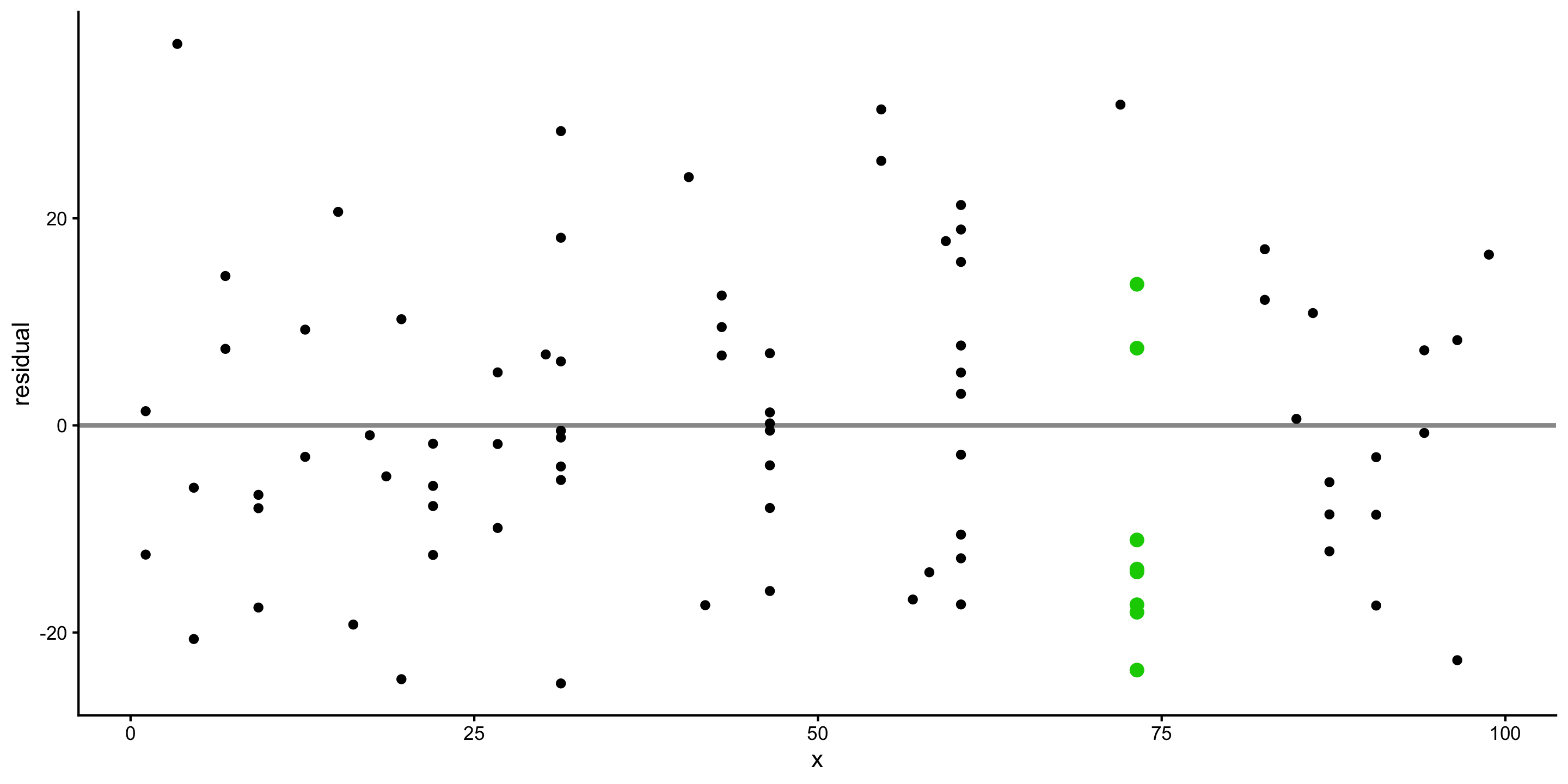
- We’ll learn to use different residual plots to more formally assess linear model assumptions
Activity: Extra practice interpreting coefficients
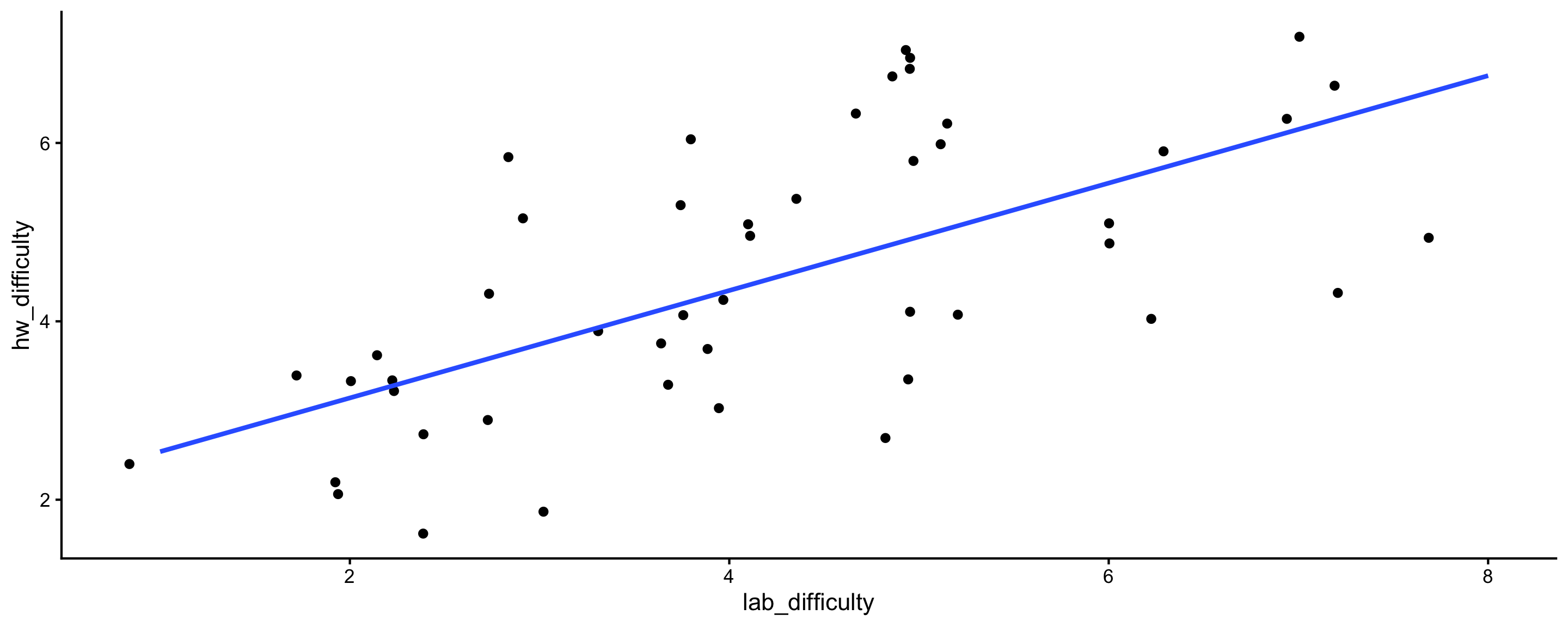
- Q1: How should we interpret the intercept?
- Q2: How should we interpret the coefficient on
lab_difficulty?