Summary Statistics

Megan Ayers

Math 141 | Spring 2026
Monday, Week 2

Announcements

The teaching team would love to see you in office hours!
- Megan’s office hours: For individual or small group help on problems or concepts
- Course assistant office hours: To work on assignments with your peers and get help from the course assistants when you are stuck

Reminder: If you haven’t already, make sure your access to Gradescope is set up.
Please select pages for each problem part on Gradescope

Last Time

Learned about the structure of ggplot2
Learn five standard graphs for numerical/quantitative data: histograms, boxplots, barplots, scatterplots, and linegraphs

Goals for Today

Consider measures for summarizing quantitative data
- Center
- Spread/variability
Consider measures for summarizing categorical data
- Contingency tables

Import the Data

biketown <- read.csv("data/biketown.csv")

# Inspect the data
str(biketown)

'data.frame':   9999 obs. of  19 variables:
 $ RouteID         : int  4074085 3719219 3789757 3576798 3459987 3947695 3549550 4411957 4098004 4096862 ...
 $ PaymentPlan     : chr  "Subscriber" "Casual" "Casual" "Subscriber" ...
 $ StartHub        : chr  "SE Elliott at Division" "SW Yamhill at Director Park" "NE Holladay at MLK" "NW Couch at 2nd" ...
 $ StartLatitude   : num  45.5 45.5 45.5 45.5 45.5 ...
 $ StartLongitude  : num  -123 -123 -123 -123 -123 ...
 $ StartDate       : chr  "8/17/2017" "7/22/2017" "7/27/2017" "7/12/2017" ...
 $ StartTime       : chr  "10:44:00" "14:49:00" "14:13:00" "13:23:00" ...
 $ EndHub          : chr  "Blues Fest - SW Waterfront at Clay - Disabled" "SW 2nd at Pine" "NE Alberta at NE 29th/30th - Community Corral" "NW Raleigh at 21st" ...
 $ EndLatitude     : num  45.5 45.5 45.6 45.5 45.5 ...
 $ EndLongitude    : num  -123 -123 -123 -123 -123 ...
 $ EndDate         : chr  "8/17/2017" "7/22/2017" "7/27/2017" "7/12/2017" ...
 $ EndTime         : chr  "10:56:00" "15:00:00" "14:42:00" "13:38:00" ...
 $ TripType        : logi  NA NA NA NA NA NA ...
 $ BikeID          : int  6163 6843 6409 7375 6354 6088 6089 5988 6857 6847 ...
 $ BikeName        : chr  "0488 BIKETOWN" "0759 BIKETOWN" "0614 BIKETOWN" "0959 BETRUE MAX - RECON" ...
 $ Distance_Miles  : num  1.91 0.72 3.42 1.81 4.51 5.54 1.59 1.03 0.7 1.72 ...
 $ Duration        : num  11.5 11.4 28.3 14.9 60.5 ...
 $ RentalAccessPath: chr  "keypad" "keypad" "keypad" "keypad" ...
 $ MultipleRental  : logi  FALSE FALSE FALSE FALSE TRUE FALSE ...

Summarizing Data

	RouteID	PaymentPlan	StartHub	Distance_Miles
25	3596434	Subscriber	NW 18th at Flanders	0.59
26	3607170	Subscriber	NW Raleigh at 21st	0.71
27	3631639	Casual	SW 2nd at Pine	3.15
28	3912181	Casual	SE Water at Taylor	5.89
29	4031739	Casual	SE Clay at Water	1.34
30	3859969	Casual	SW Naito at Morrison	1.56
31	4315016	Casual	NW Everett at 22nd	3.50
32	4252609	Casual	NW Flanders at 14th	1.81
33	3809564	Casual	NA	2.74

Hard to do by eyeballing a spreadsheet with many rows!

Summarizing Data Visually

For a quantitative variable, often want to answer:

What is an average value?
What is the trend/shape of the variable?
How much variation is there from case to case?

Need to learn key summary statistics: Numerical values computed based on the observed cases.

Measures of Center

Mean: Average of all the observations

\(n\) = Number of cases (sample size)
\(x_i\) = value of the i-th observation
Denote by \(\bar{x}\)

Measures of Center

Mean: Average of all the observations

\(n\) = Number of cases (sample size)
\(x_i\) = value of the i-th observation
Denote by \(\bar{x}\)

\[ \bar{x} = \frac{1}{n} \sum_{i = 1}^n x_i \]

Measures of Center

Mean: Average of all the observations

\(n\) = Number of cases (sample size)
\(x_i\) = value of the i-th observation
Denote by \(\bar{x}\)

\[ \bar{x} = \frac{1}{n} \sum_{i = 1}^n x_i \]

# Test out on first 6 values
head(biketown$Distance_Miles)

[1] 1.91 0.72 3.42 1.81 4.51 5.54

(1.91 + 0.72 + 3.42 + 1.81 + 4.51 + 5.54) / 6

[1] 2.985

# Compute in R for all values
mean(biketown$Distance_Miles)

[1] 2.044768

Measures of Center

Median: Middle value

Half of the data falls below the median
Denote by \(m\)
If \(n\) is even, then it is the average of the middle two values

Measures of Center

Median: Middle value

Half of the data falls below the median
Denote by \(m\)
If \(n\) is even, then it is the average of the middle two values

# Test out on first 6 values
head(biketown$Distance_Miles)

[1] 1.91 0.72 3.42 1.81 4.51 5.54

sort(head(biketown$Distance_Miles))

[1] 0.72 1.81 1.91 3.42 4.51 5.54

(3.42 + 1.91) / 2

[1] 2.665

Compute in R:

median(biketown$Distance_Miles)

[1] 1.48

Measures of Center

Q: Why is the mean larger than the median?

data.frame(mean_miles = mean(biketown$Distance_Miles),
           median_miles = median(biketown$Distance_Miles))

  mean_miles median_miles
1   2.044768         1.48

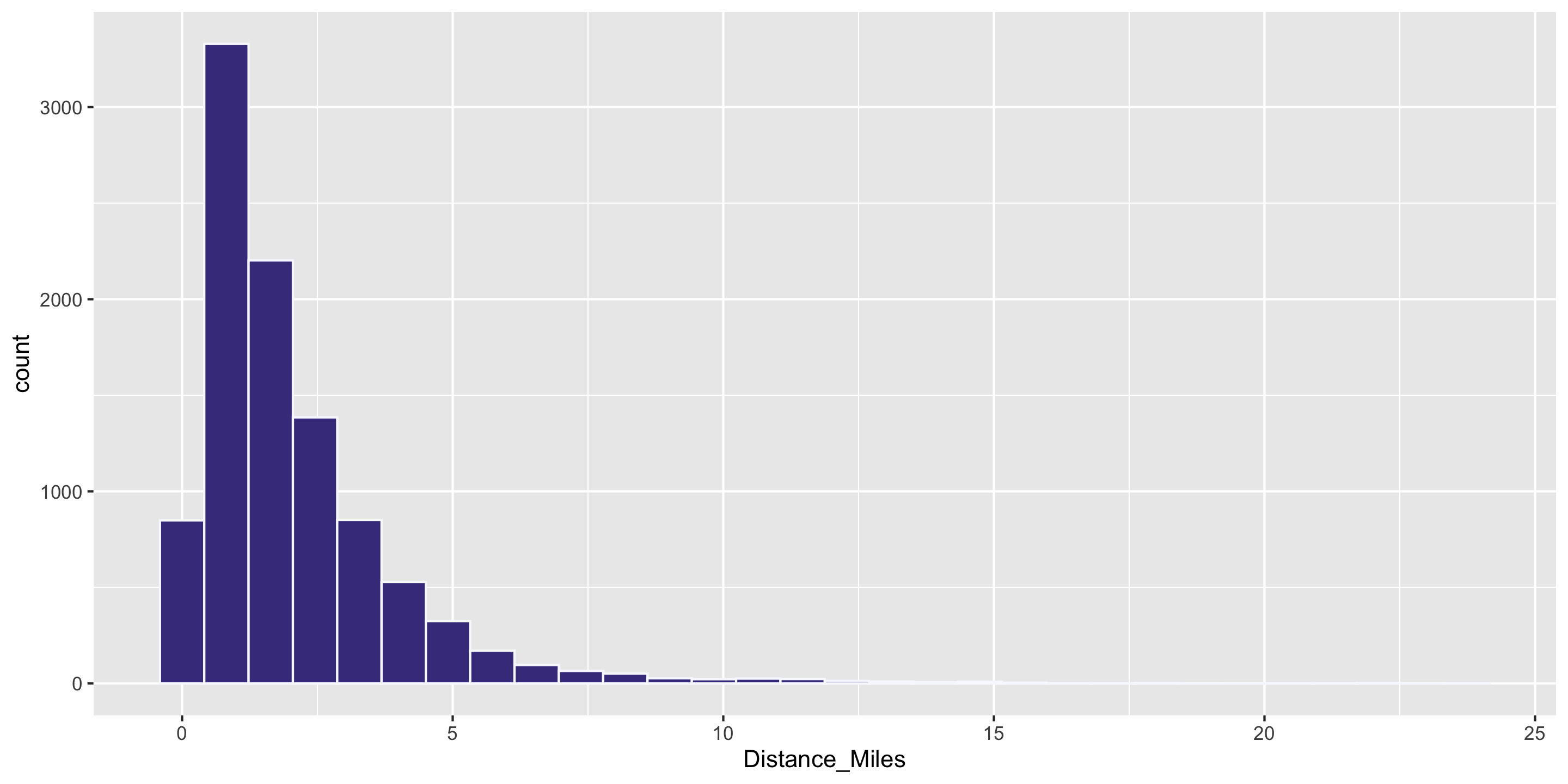
Answer: the distribution is skewed. In skewed distributions, the mean is pulled farther in the direction of skew than the median.

Measures of Center

Note: The mean is very sensitive to outliers, while the median is not.

my_data <- c(1, 2, 5, 7, 8, 10)
my_data_with_outlier <- c(1, 2, 5, 7, 8, 100)

mean(my_data)

[1] 5.5

mean(my_data_with_outlier)

[1] 20.5

median(my_data)

[1] 6

median(my_data_with_outlier)

[1] 6

We call the median a robust statistic.

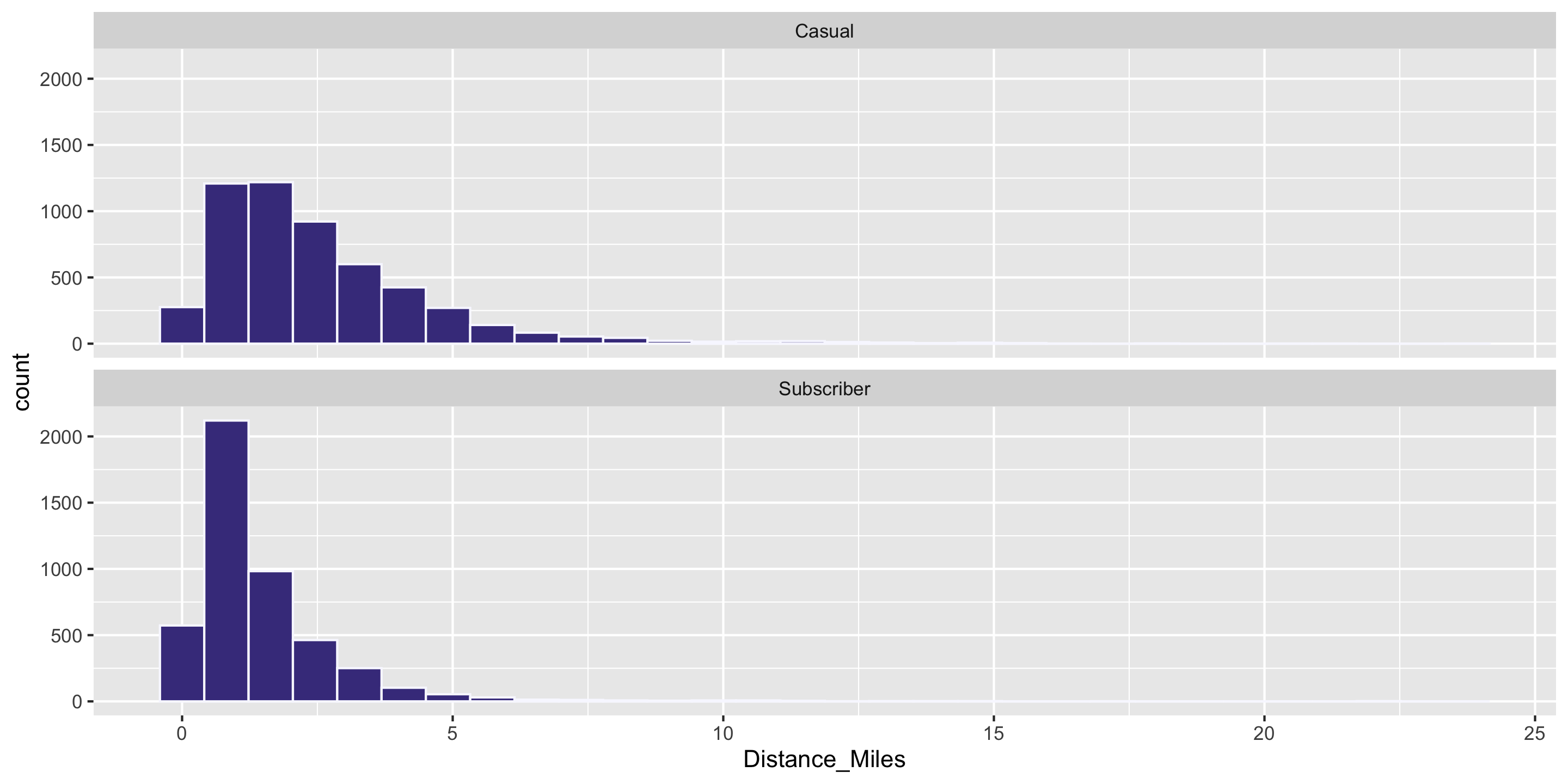
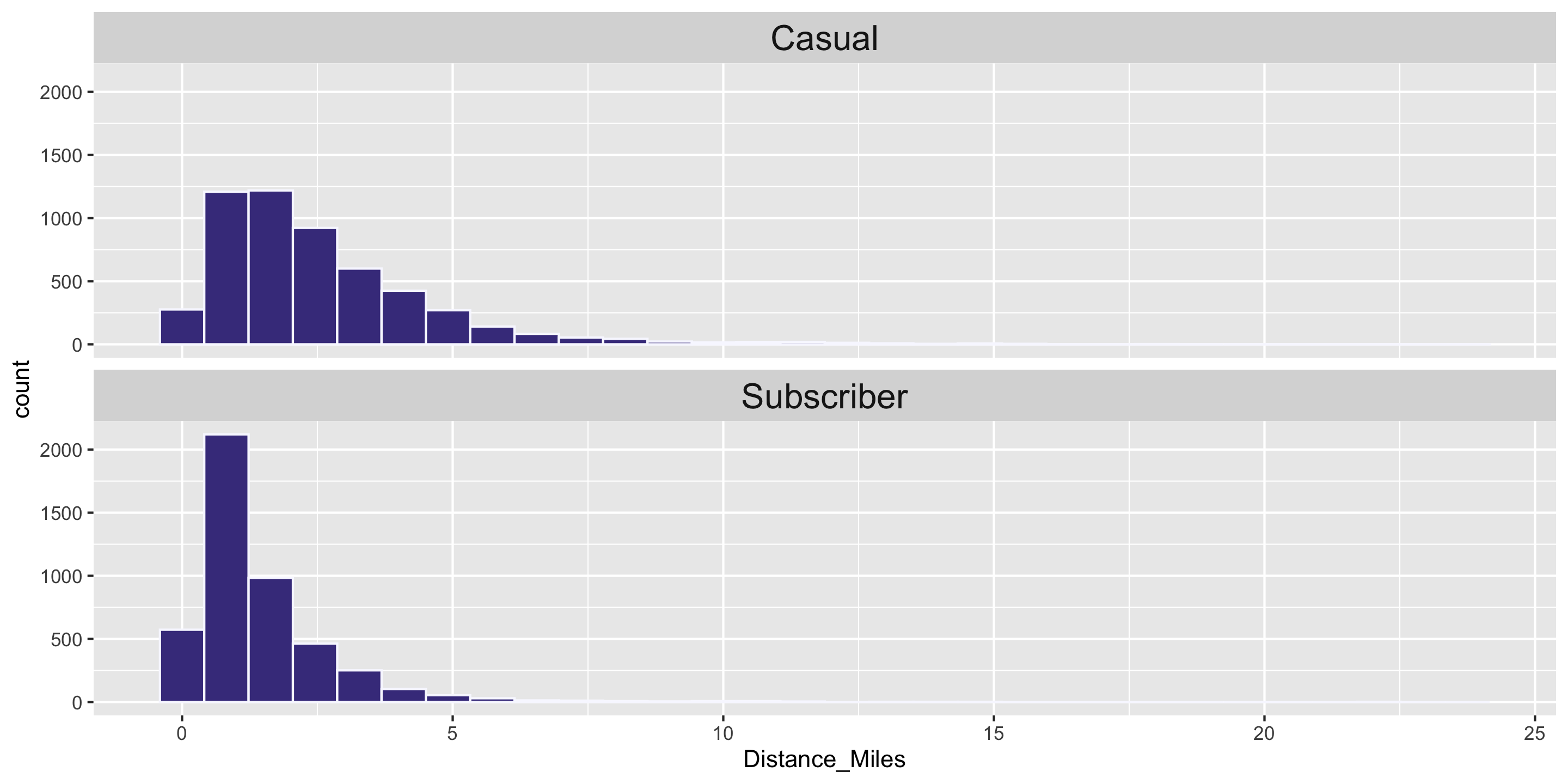
Computing Measures of Center by Groups

Question: Who travels further, on average? Casual biketown users or payment plan subscribers?

Computing Measures of Center by Groups

Handy dplyr functions that we’ll learn: group_by() and summarize().

library(dplyr)

# Calculate group *MEANS*
biketown %>%
  group_by(PaymentPlan) %>%
  summarize(mean_dist = mean(Distance_Miles))

# A tibble: 2 × 2
  PaymentPlan mean_dist
  <chr>           <dbl>
1 Casual           2.56
2 Subscriber       1.45

# Calculate group *MEDIANS*
biketown %>%
  group_by(PaymentPlan) %>%
  summarize(median_dist = median(Distance_Miles))

# A tibble: 2 × 2
  PaymentPlan median_dist
  <chr>             <dbl>
1 Casual             2.03
2 Subscriber         1.02

Measures of Variability

Want a statistic that captures how much observations deviate from the mean

Find how much each observation deviates from the mean.
Idea: Compute the average of the deviations

Measures of Variability

Want a statistic that captures how much observations deviate from the mean

Find how much each observation deviates from the mean.
Idea: Compute the average of the deviations

\[ \frac{1}{n} \sum_{i = 1}^n (x_i - \bar{x}) \]

Measures of Variability

Want a statistic that captures how much observations deviate from the mean

Find how much each observation deviates from the mean.
Idea: Compute the average of the deviations

\[ \frac{1}{n} \sum_{i = 1}^n (x_i - \bar{x}) \]

# Test out on first 6 values
head(biketown$Distance_Miles)

[1] 1.91 0.72 3.42 1.81 4.51 5.54

Problem?

# Calculate mean by hand
(1.91 + 0.72 + 3.42 + 1.81 + 4.51 + 5.54) / 6

[1] 2.985

# Calculate average deviations by hand
((1.91 - 2.985) + (0.72 - 2.985) + 
  (3.42 - 2.985) + (1.81 - 2.985) +
  (4.51 - 2.985) + (5.54 - 2.985)) / 6

[1] 0

Measures of Variability

Want a statistic that captures how much observations deviate from the mean

NEW proposal:

Find how much each observation deviates from the mean.
Compute the average of the squared deviations.

Measures of Variability

Want a statistic that captures how much observations deviate from the mean

NEW proposal:

Find how much each observation deviates from the mean.
Compute the average of the squared deviations.

# Test out on first 6 values
head(biketown$Distance_Miles)

[1] 1.91 0.72 3.42 1.81 4.51 5.54

# Calculate mean by hand
(1.91 + 0.72 + 3.42 + 1.81 + 4.51 + 5.54) / 6

[1] 2.985

# Calculate average squared deviations by hand
((1.91 - 2.985)^2 + (0.72 - 2.985)^2 + 
  (3.42 - 2.985)^2 + (1.81 - 2.985)^2 +
  (4.51 - 2.985)^2 + (5.54 - 2.985)^2) / 6

[1] 2.784892

Measures of Variability

Want a statistic that captures how much observations deviate from the mean

NEW proposal, formula:

Find how much each observation deviates from the mean.
Compute the (nearly) average of the squared deviations.
Called sample variance \(s^2\).

Measures of Variability

Want a statistic that captures how much observations deviate from the mean

NEW proposal, formula:

Find how much each observation deviates from the mean.
Compute the (nearly) average of the squared deviations.
Called sample variance \(s^2\).

\[ s^2 = \frac{1}{n - 1} \sum_{i = 1}^n (x_i - \bar{x})^2 \]

We’ll learn why we divide by \(n-1\) instead of \(n\) later in the course.

Measures of Variability

Want a statistic that captures how much observations deviate from the mean

NEW proposal, formula:

Find how much each observation deviates from the mean.
Compute the (nearly) average of the squared deviations.
Called sample variance \(s^2\).

\[ s^2 = \frac{1}{n - 1} \sum_{i = 1}^n (x_i - \bar{x})^2 \]

We’ll learn why we divide by \(n-1\) instead of \(n\) later in the course.

Compute with R:

var(biketown$Distance_Miles)

[1] 3.805638

Measures of Variability

Want a statistic that captures how much observations deviate from the mean

Find how much each observation deviates from the mean.
Compute the (nearly) average of the squared deviations (\(s^2\)).
Because observations are squared, units differ from original data.

The square root of the sample variance is called the sample standard deviation \(s\).

Compute in R:

var(biketown$Distance_Miles)  # Variance

[1] 3.805638

sd(biketown$Distance_Miles)   # Standard deviation

[1] 1.950804

sqrt(var(biketown$Distance_Miles))

[1] 1.950804

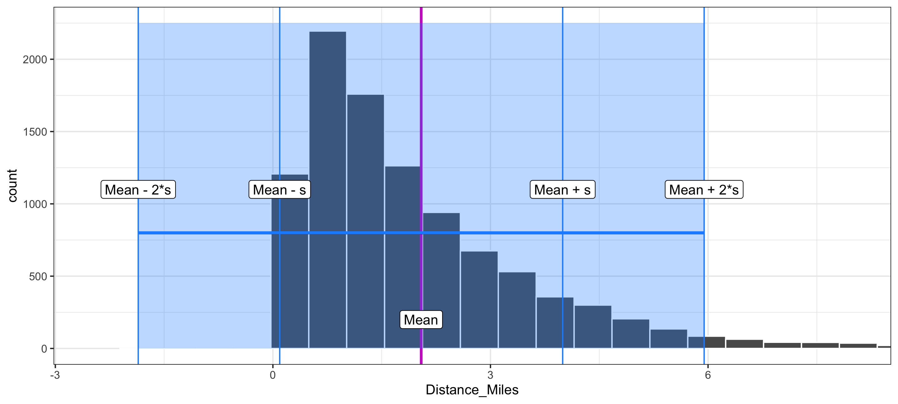
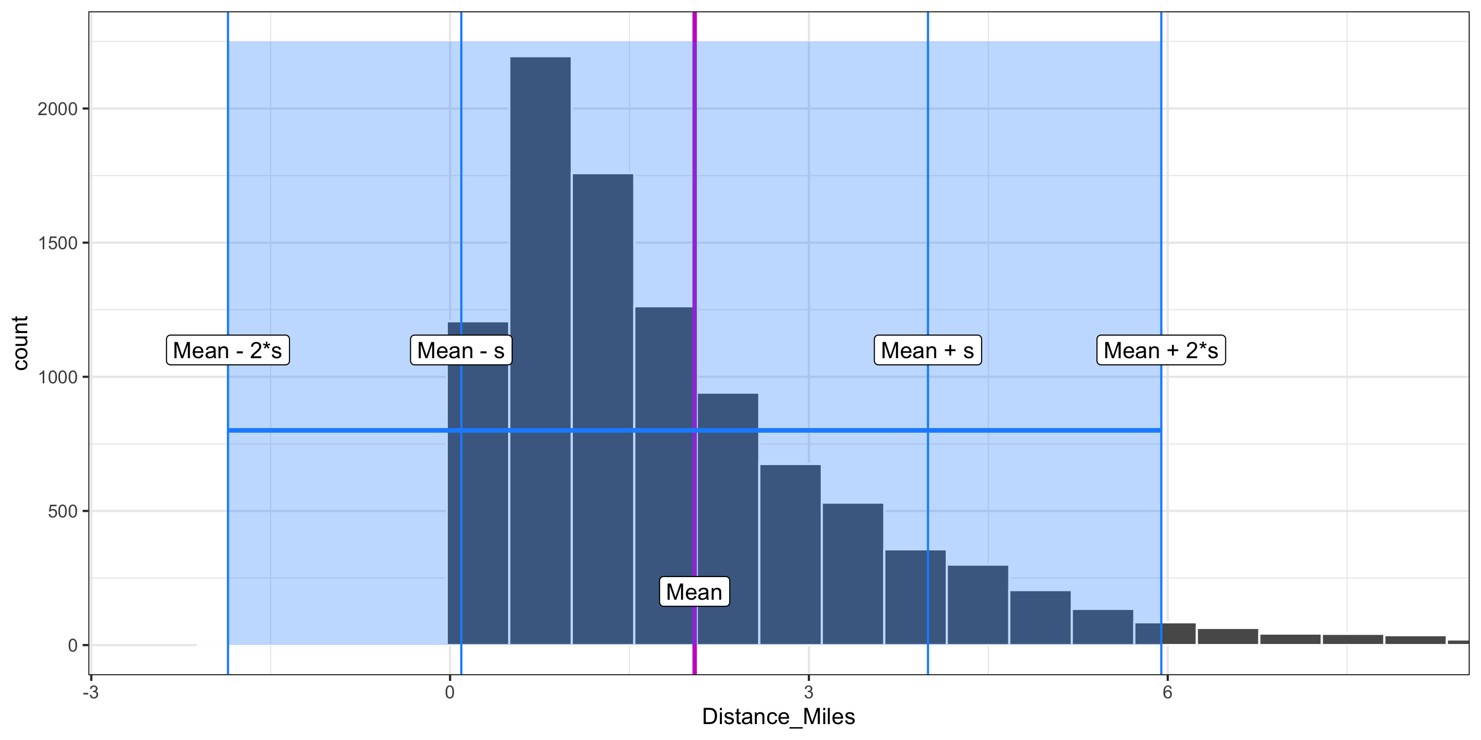
Visualizing Standard Deviation

The standard deviation measures the typical size of deviations from the mean.
For most data sets, the large majority of observations are within 2 standard deviations of the mean.

sd(biketown$Distance_Miles)

[1] 1.950804

Measures of Variability

In addition to the sample standard deviation and the sample variance, there is the sample interquartile range (IQR):

\[ \mbox{IQR} = \mbox{Q}_3 - \mbox{Q}_1 \]

25% of all observations are less than the first quartile Q1
25% of all observations are greater than the third quartile Q3

Compute with R:

IQR(biketown$Distance_Miles)

[1] 1.89

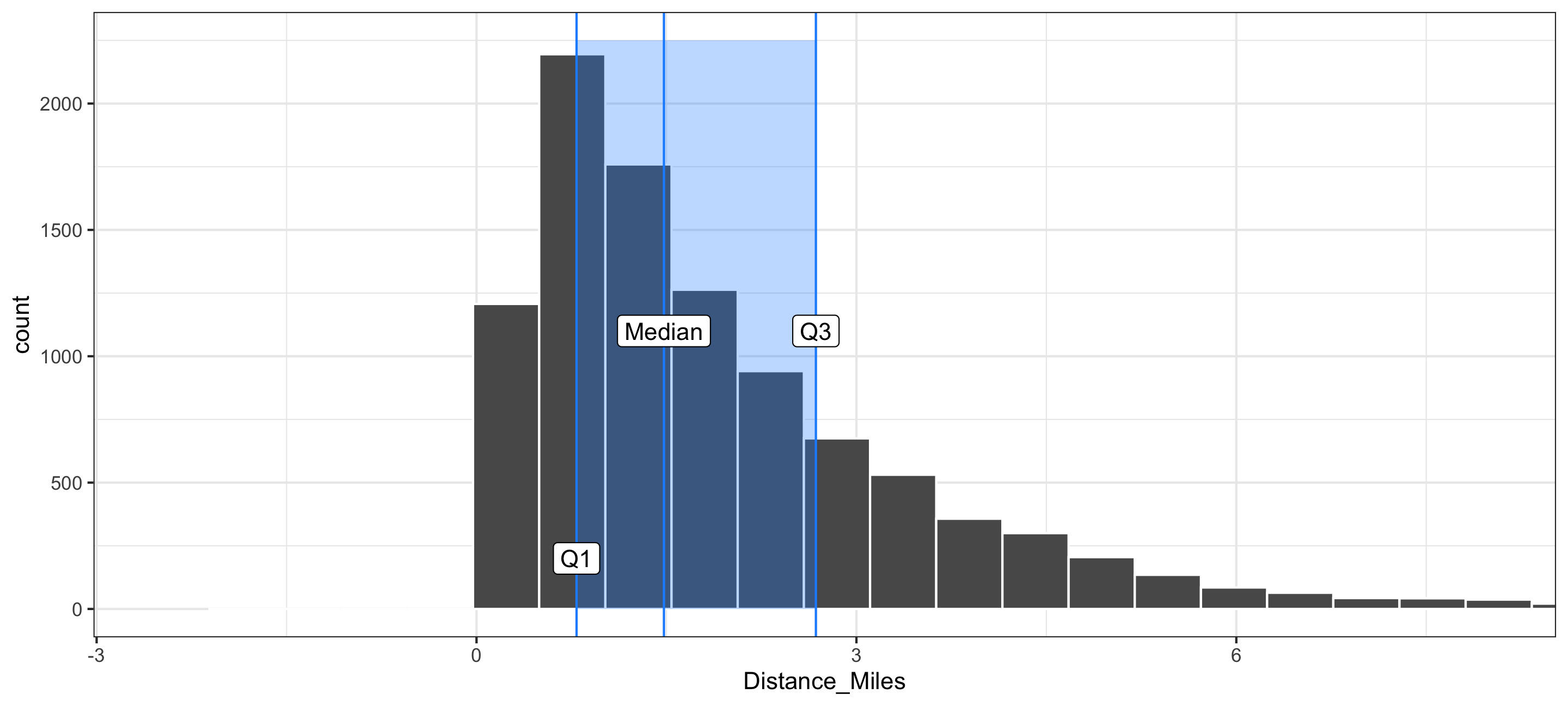
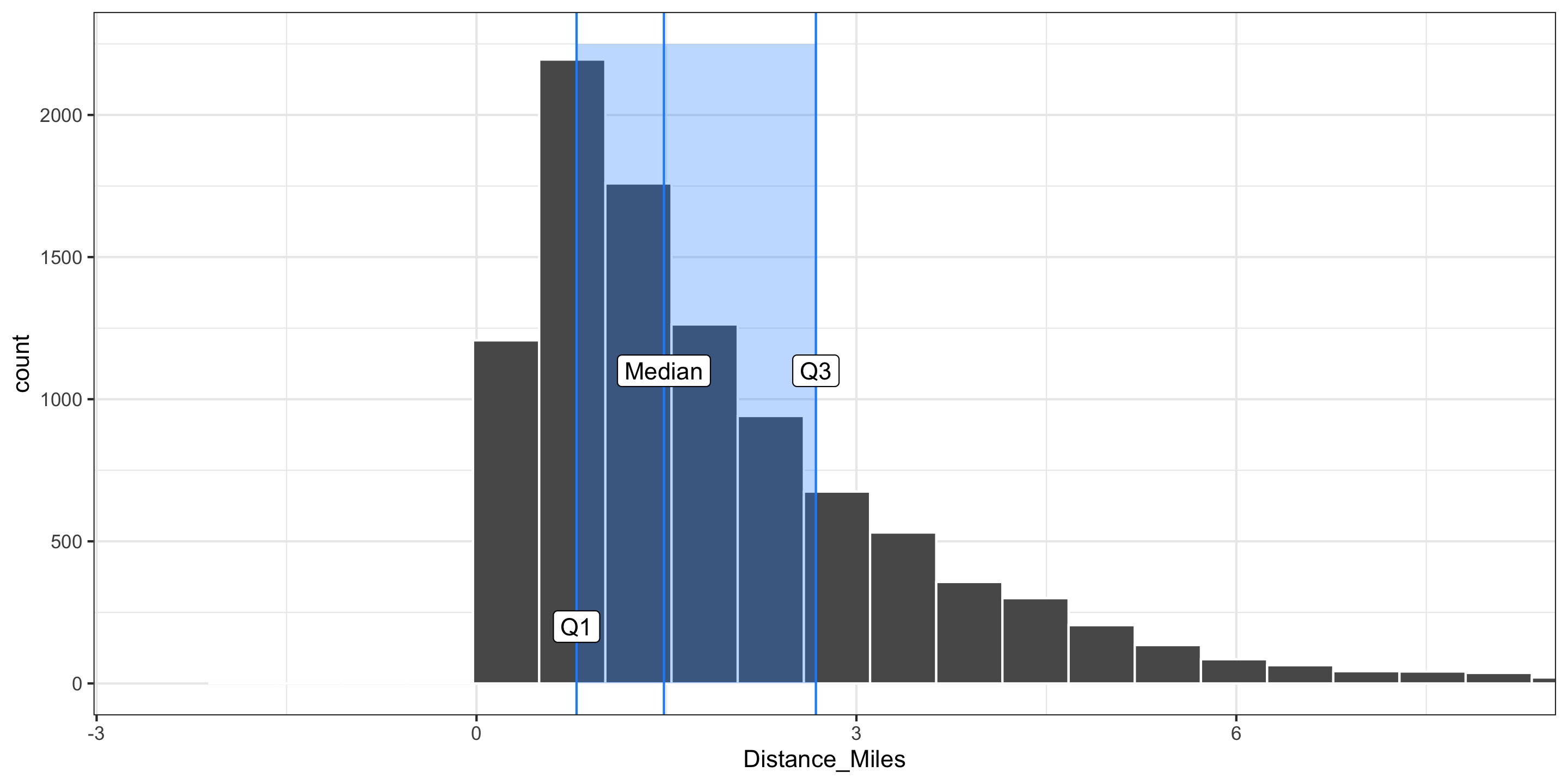
Visualizing the IQR

In addition to the sample standard deviation and the sample variance, there is the sample interquartile range (IQR):

\[ \mbox{IQR} = \mbox{Q}_3 - \mbox{Q}_1 \]

quantile(biketown$Distance_Miles, c(0.25, 0.5, 0.75))

 25%  50%  75% 
0.79 1.48 2.68

Comparing Measures of Variability

Q: Which is more robust to outliers, the IQR or \(s\)?

Q: Which is more commonly used, the IQR or \(s\)?

Summarizing Categorical Variables

New data set: Cambridge dogs

dogs <- read.csv("https://data.cambridgema.gov/api/views/sckh-3xyx/rows.csv")
str(dogs)

'data.frame':   1581 obs. of  6 variables:
 $ Dog_Name        : chr  "Thor" "Lucy" "Ruby" "Georgie" ...
 $ Dog_Breed       : chr  "Boxer" "Poodle" "Collie" "Lhasa Apso" ...
 $ Location_masked : logi  NA NA NA NA NA NA ...
 $ Latitude_masked : num  42.4 42.4 42.4 42.4 42.4 ...
 $ Longitude_masked: num  -71.1 -71.1 -71.1 -71.1 -71.1 ...
 $ Neighborhood    : chr  "East Cambridge" "Mid-Cambridge" "Neighborhood Nine" "West Cambridge" ...

Cambridge dogs data set

May want to focus on the dogs with the 5 most common names

dogs <- read.csv("https://data.cambridgema.gov/api/views/sckh-3xyx/rows.csv")

# Useful wrangling that we will come back to
dogs_top5 <- dogs %>%
  mutate(Breed = case_when(Dog_Breed == "Mixed Breed" ~ "Mixed",
                           TRUE ~ "Single")) %>%
  filter(Dog_Name %in% c("Luna", "Charlie", "Lucy", "Cooper", "Rosie"))


head(dogs_top5)

  Dog_Name                  Dog_Breed Location_masked Latitude_masked
1     Lucy                     Poodle              NA         42.3696
2     Luna                LABRADOODLE              NA         42.3860
3  Charlie         Border Terrier Mix              NA         42.3596
4   Cooper German Shorthaired Pointer              NA         42.3573
5  Charlie           Golden Retriever              NA         42.3895
6     Luna                Mixed Breed              NA         42.3913
  Longitude_masked      Neighborhood  Breed
1         -71.1109     Mid-Cambridge Single
2         -71.1362 Neighborhood Nine Single
3         -71.1143     Cambridgeport Single
4         -71.1015     Cambridgeport Single
5         -71.1311 Neighborhood Nine Single
6         -71.1329   North Cambridge  Mixed

Frequency Table

Distributions of categorical variables can be presented in tables and summarized in bar charts.

count(dogs_top5, Dog_Name)  # Handy function

  Dog_Name  n
1  Charlie 14
2   Cooper  8
3     Lucy 10
4     Luna 14
5    Rosie 10

ggplot(data = dogs_top5, 
    mapping = aes(x = Dog_Name)) +
  geom_bar()

Q: Why can’t we use mean or standard deviation here?

Another `ggplot2` `geom`: `geom_col()`

If you have already aggregated the data, you will use geom_col() instead of geom_bar().

dog_counts <- count(dogs_top5, Dog_Name)
dog_counts

  Dog_Name  n
1  Charlie 14
2   Cooper  8
3     Lucy 10
4     Luna 14
5    Rosie 10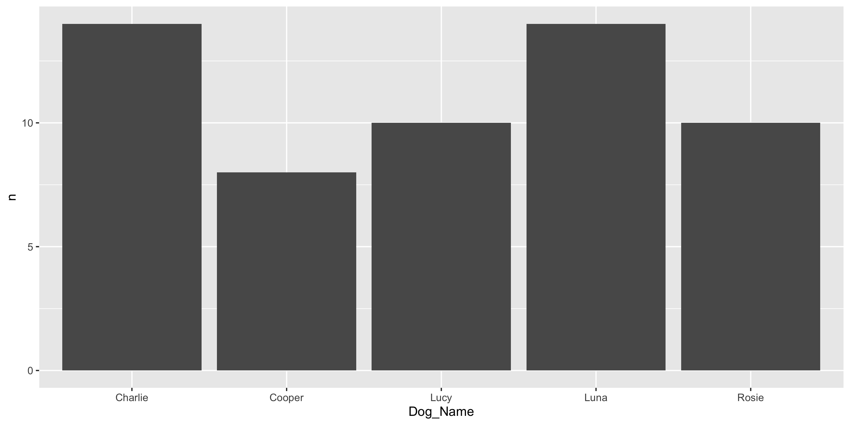

ggplot(data = dog_counts,
       mapping = aes(x = Dog_Name,
                     y = n)) +
  geom_col()

Another `ggplot2` `geom`: `geom_col()`

And you can use fct_reorder to order bars by value

dog_counts <- count(dogs_top5, Dog_Name)
dog_counts

  Dog_Name  n
1  Charlie 14
2   Cooper  8
3     Lucy 10
4     Luna 14
5    Rosie 10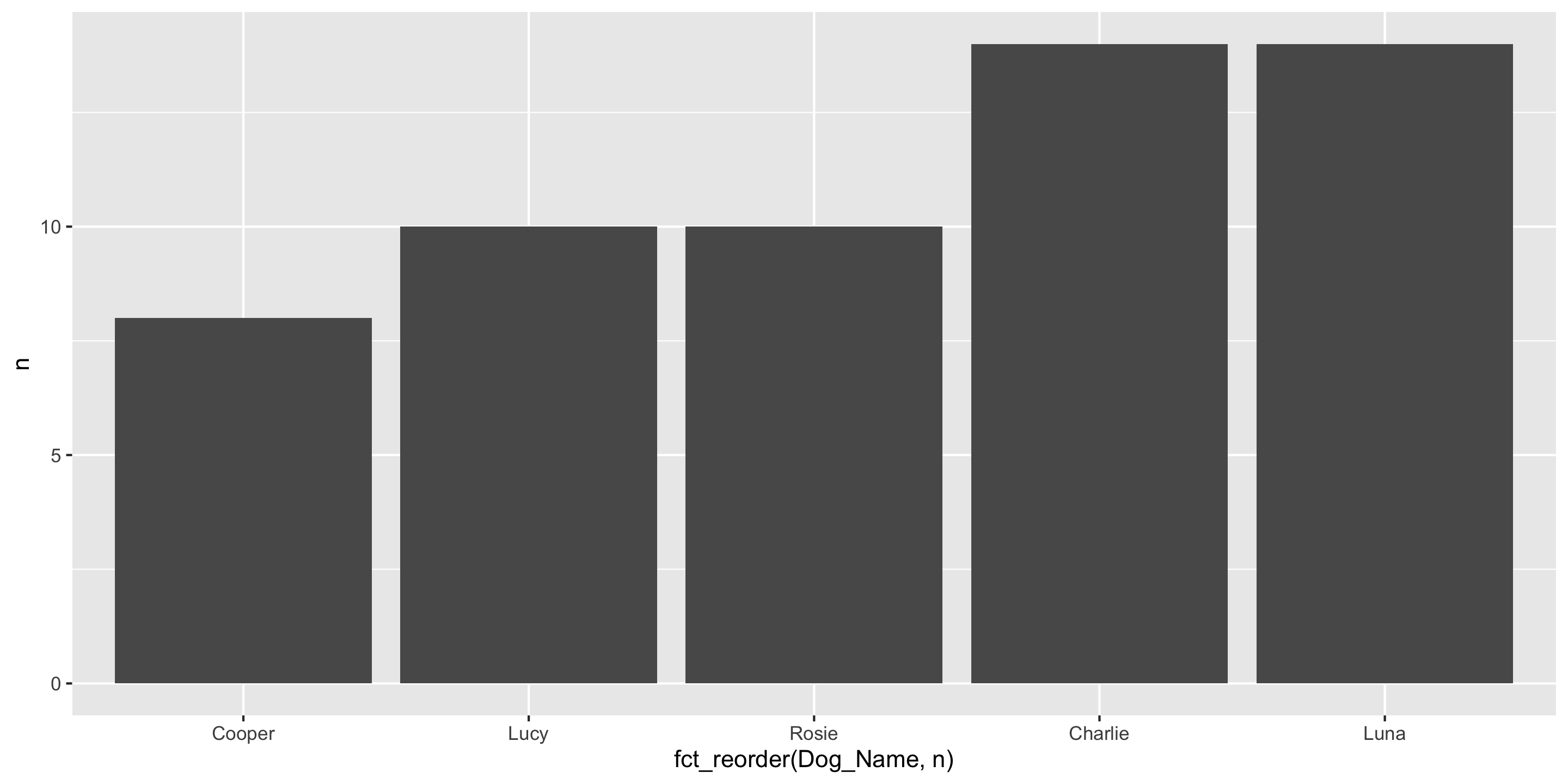

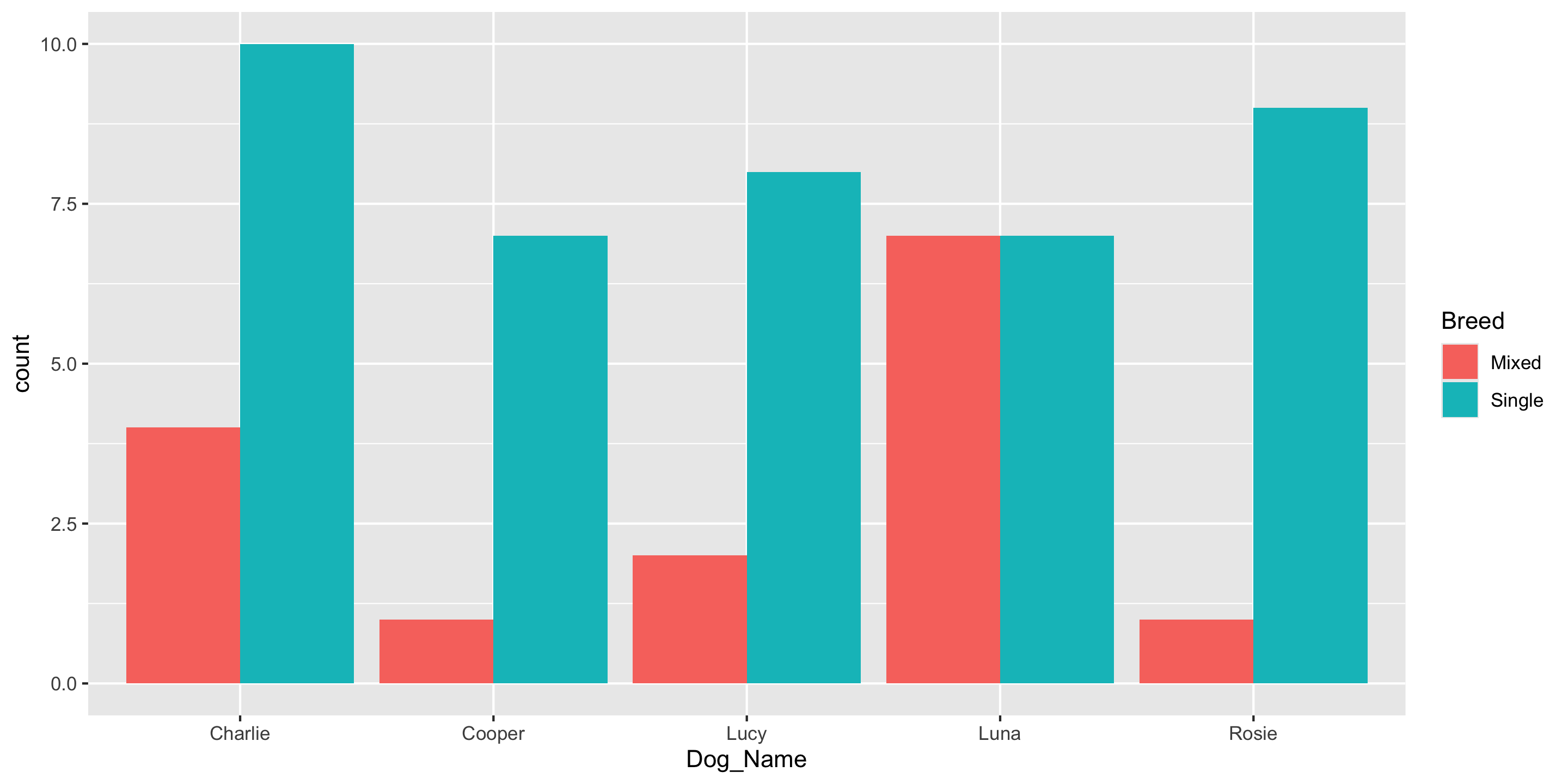
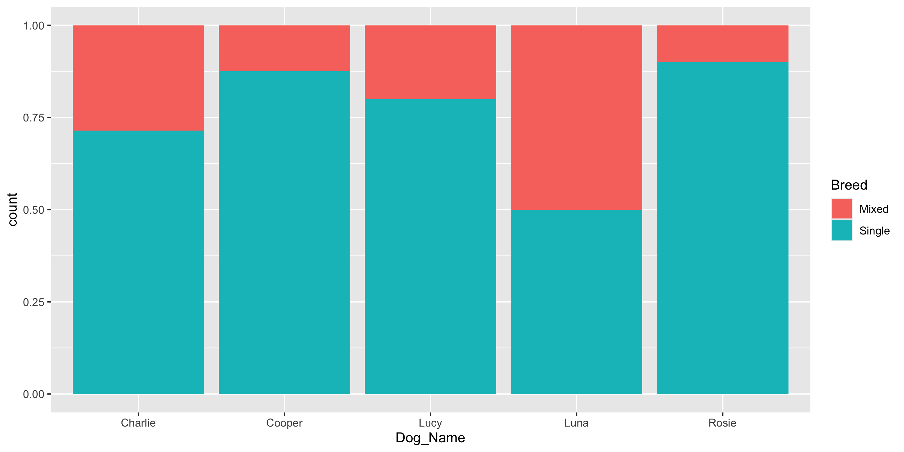
library(forcats)
ggplot(data = dog_counts,
       mapping = aes(x = fct_reorder(Dog_Name, n),
                     y = n)) +
  geom_col()

Contingency Table

To compare 2 categorical variables, we can use a contingency table

# Using `count()` from dplyr
count(dogs_top5, Dog_Name, Breed)

   Dog_Name  Breed  n
1   Charlie  Mixed  4
2   Charlie Single 10
3    Cooper  Mixed  1
4    Cooper Single  7
5      Lucy  Mixed  2
6      Lucy Single  8
7      Luna  Mixed  7
8      Luna Single  7
9     Rosie  Mixed  1
10    Rosie Single  9

# More common presentation
table(dogs_top5$Dog_Name, dogs_top5$Breed)

         
          Mixed Single
  Charlie     4     10
  Cooper      1      7
  Lucy        2      8
  Luna        7      7
  Rosie       1      9

ggplot(data = dogs_top5, 
    mapping = aes(x = Dog_Name, fill = Breed)) +
  geom_bar(position = "dodge")

Conditional Proportions

Beyond raw counts, we often summarize categorical data with conditional proportions.
- Especially when looking for relationships!

ggplot(data = dogs_top5, 
    mapping = aes(x = Dog_Name, fill = Breed)) +
  geom_bar(position = "fill")

Conditional Proportions

count(dogs_top5, Dog_Name, Breed)

   Dog_Name  Breed  n
1   Charlie  Mixed  4
2   Charlie Single 10
3    Cooper  Mixed  1
4    Cooper Single  7
5      Lucy  Mixed  2
6      Lucy Single  8
7      Luna  Mixed  7
8      Luna Single  7
9     Rosie  Mixed  1
10    Rosie Single  9

count(dogs_top5, Dog_Name, Breed) %>%
  group_by(Dog_Name) %>%     ## Conditions on Dog Name
  mutate(prop = n / sum(n))  ## Adds/changes columns

# A tibble: 10 × 4
# Groups:   Dog_Name [5]
   Dog_Name Breed      n  prop
   <chr>    <chr>  <int> <dbl>
 1 Charlie  Mixed      4 0.286
 2 Charlie  Single    10 0.714
 3 Cooper   Mixed      1 0.125
 4 Cooper   Single     7 0.875
 5 Lucy     Mixed      2 0.2  
 6 Lucy     Single     8 0.8  
 7 Luna     Mixed      7 0.5  
 8 Luna     Single     7 0.5  
 9 Rosie    Mixed      1 0.1  
10 Rosie    Single     9 0.9

We’ll go over these data wrangling functions on Wednesday!

Conditional Proportions

count(dogs_top5, Dog_Name, Breed) %>%
  group_by(Dog_Name) %>%     ## Conditions on Dog Name
  mutate(prop = n / sum(n))  ## Adds/changes columns

# A tibble: 10 × 4
# Groups:   Dog_Name [5]
   Dog_Name Breed      n  prop
   <chr>    <chr>  <int> <dbl>
 1 Charlie  Mixed      4 0.286
 2 Charlie  Single    10 0.714
 3 Cooper   Mixed      1 0.125
 4 Cooper   Single     7 0.875
 5 Lucy     Mixed      2 0.2  
 6 Lucy     Single     8 0.8  
 7 Luna     Mixed      7 0.5  
 8 Luna     Single     7 0.5  
 9 Rosie    Mixed      1 0.1  
10 Rosie    Single     9 0.9

count(dogs_top5, Dog_Name, Breed) %>%
  group_by(Breed) %>%     ## Conditions on Breed
  mutate(prop = n / sum(n))  ## Adds/changes columns

# A tibble: 10 × 4
# Groups:   Breed [2]
   Dog_Name Breed      n   prop
   <chr>    <chr>  <int>  <dbl>
 1 Charlie  Mixed      4 0.267 
 2 Charlie  Single    10 0.244 
 3 Cooper   Mixed      1 0.0667
 4 Cooper   Single     7 0.171 
 5 Lucy     Mixed      2 0.133 
 6 Lucy     Single     8 0.195 
 7 Luna     Mixed      7 0.467 
 8 Luna     Single     7 0.171 
 9 Rosie    Mixed      1 0.0667
10 Rosie    Single     9 0.220

Q: How does the interpretation change based on which variable you condition on?

Reminders

The teaching team would love to see you in office hours!
Next time:
- We’ll define data wrangling and
- Learn to use more functions and methods to summarize and wrangle data

Announcements

Last Time

Goals for Today

Import the Data

Summarizing Data

Summarizing Data Visually

Measures of Center

Measures of Center

Measures of Center

Measures of Center

Measures of Center

Measures of Center

Measures of Center

Computing Measures of Center by Groups

Computing Measures of Center by Groups

Measures of Variability

Measures of Variability

Measures of Variability

Measures of Variability

Measures of Variability

Measures of Variability

Measures of Variability

Measures of Variability

Measures of Variability

Visualizing Standard Deviation

Measures of Variability

Visualizing the IQR

Comparing Measures of Variability

Summarizing Categorical Variables

New data set: Cambridge dogs

Cambridge dogs data set

Frequency Table

Another ggplot2 geom: geom_col()

Another ggplot2 geom: geom_col()

Contingency Table

Conditional Proportions

Conditional Proportions

Conditional Proportions

Reminders

Another `ggplot2` `geom`: `geom_col()`

Another `ggplot2` `geom`: `geom_col()`