Data Visualization: the 5 Named Graphs with ggplot2

Megan Ayers

Math 141 | Spring 2026
Friday, Week 1

Reminders/Announcements

• If you plan to request academic accommodations, please submit these through the DAR student portal
• Course assistant office hours are now on Moodle
• The DataLab @ Reed
• First homework assignment is posted!

Last Time

• Data frames
• Motivation for data visualizations
• “Grammar” of graphics and good graphical practices

Goals for Today

• Recall our motivation for good graphics
• Learn the general structure of ggplot2
• Learn five standard graphs for numerical/quantitative data:
  • Histogram: one numerical variable
  • Boxplot: one numerical variable
  • Barplot: one numerical variable and at least one categorical variable
  • Scatterplot and Linegraph: two numerical variables

Load Necessary Packages

ggplot2 is part of this collection of data science packages.

# Load necessary packages
library(tidyverse)

Also, above is an example of a code comment: # Load necessary packages

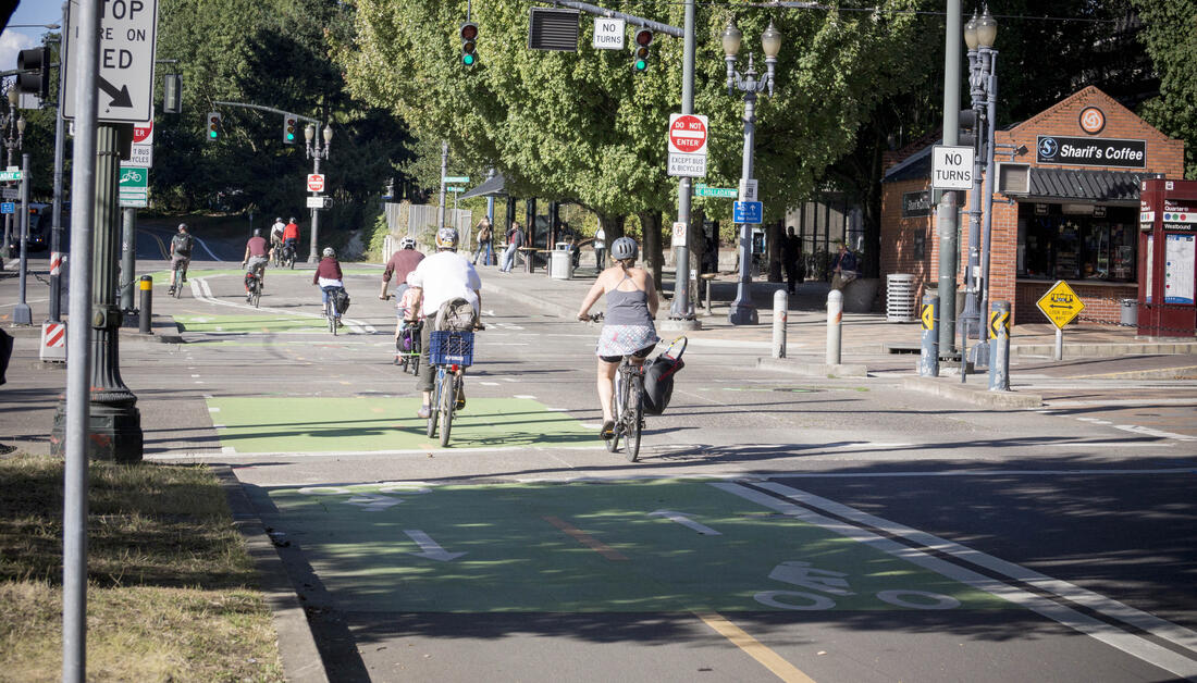
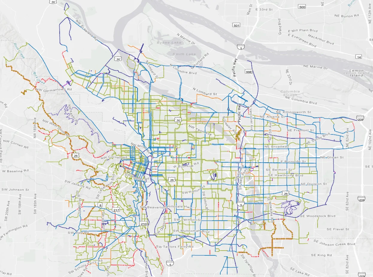
Data Setting: Portland Bikeshare Data

Import the Data

biketown <- read.csv("data/biketown.csv")

# Inspect the data
glimpse(biketown)

Rows: 9,999
Columns: 19
$ RouteID          <int> 4074085, 3719219, 3789757, 3576798, 3459987, 3947695,…
$ PaymentPlan      <chr> "Subscriber", "Casual", "Casual", "Subscriber", "Casu…
$ StartHub         <chr> "SE Elliott at Division", "SW Yamhill at Director Par…
$ StartLatitude    <dbl> 45.50513, 45.51898, 45.52990, 45.52389, 45.53028, 45.…
$ StartLongitude   <dbl> -122.6534, -122.6813, -122.6628, -122.6722, -122.6547…
$ StartDate        <chr> "8/17/2017", "7/22/2017", "7/27/2017", "7/12/2017", "…
$ StartTime        <chr> "10:44:00", "14:49:00", "14:13:00", "13:23:00", "19:3…
$ EndHub           <chr> "Blues Fest - SW Waterfront at Clay - Disabled", "SW …
$ EndLatitude      <dbl> 45.51287, 45.52142, 45.55902, 45.53409, 45.52990, 45.…
$ EndLongitude     <dbl> -122.6749, -122.6726, -122.6355, -122.6949, -122.6628…
$ EndDate          <chr> "8/17/2017", "7/22/2017", "7/27/2017", "7/12/2017", "…
$ EndTime          <chr> "10:56:00", "15:00:00", "14:42:00", "13:38:00", "20:3…
$ TripType         <lgl> NA, NA, NA, NA, NA, NA, NA, NA, NA, NA, NA, NA, NA, N…
$ BikeID           <int> 6163, 6843, 6409, 7375, 6354, 6088, 6089, 5988, 6857,…
$ BikeName         <chr> "0488 BIKETOWN", "0759 BIKETOWN", "0614 BIKETOWN", "0…
$ Distance_Miles   <dbl> 1.91, 0.72, 3.42, 1.81, 4.51, 5.54, 1.59, 1.03, 0.70,…
$ Duration         <dbl> 11.500, 11.383, 28.317, 14.917, 60.517, 53.783, 23.86…
$ RentalAccessPath <chr> "keypad", "keypad", "keypad", "keypad", "keypad", "ke…
$ MultipleRental   <lgl> FALSE, FALSE, FALSE, FALSE, TRUE, FALSE, FALSE, FALSE…

Inspect the Data

# Look at first few rows
head(biketown)

  RouteID PaymentPlan                    StartHub StartLatitude StartLongitude
1 4074085  Subscriber      SE Elliott at Division      45.50513      -122.6534
2 3719219      Casual SW Yamhill at Director Park      45.51898      -122.6813
3 3789757      Casual          NE Holladay at MLK      45.52990      -122.6628
4 3576798  Subscriber             NW Couch at 2nd      45.52389      -122.6722
5 3459987      Casual    NE 11th at Holladay Park      45.53028      -122.6547
6 3947695      Casual          SW Moody at Thomas      45.49429      -122.6719
  StartDate StartTime                                        EndHub EndLatitude
1 8/17/2017  10:44:00 Blues Fest - SW Waterfront at Clay - Disabled    45.51287
2 7/22/2017  14:49:00                                SW 2nd at Pine    45.52142
3 7/27/2017  14:13:00 NE Alberta at NE 29th/30th - Community Corral    45.55902
4 7/12/2017  13:23:00                            NW Raleigh at 21st    45.53409
5  7/3/2017  19:30:00                            NE Holladay at MLK    45.52990
6  8/8/2017  10:01:00                              SW 3rd at Ankeny    45.52248
  EndLongitude   EndDate  EndTime TripType BikeID                BikeName
1    -122.6749 8/17/2017 10:56:00       NA   6163           0488 BIKETOWN
2    -122.6726 7/22/2017 15:00:00       NA   6843           0759 BIKETOWN
3    -122.6355 7/27/2017 14:42:00       NA   6409           0614 BIKETOWN
4    -122.6949 7/12/2017 13:38:00       NA   7375 0959 BETRUE MAX - RECON
5    -122.6628  7/3/2017 20:30:00       NA   6354           0374 BIKETOWN
6    -122.6733  8/8/2017 10:55:00       NA   6088           0048 BIKETOWN
  Distance_Miles Duration RentalAccessPath MultipleRental
1           1.91   11.500           keypad          FALSE
2           0.72   11.383           keypad          FALSE
3           3.42   28.317           keypad          FALSE
4           1.81   14.917           keypad          FALSE
5           4.51   60.517           keypad           TRUE
6           5.54   53.783           keypad          FALSE

What does a row represent here?

Inspect the Data

# Determine type
# To access one variable: dataset$variable
class(biketown$BikeName)

[1] "character"

class(biketown$Distance_Miles)

[1] "numeric"

class(biketown)

[1] "data.frame"

Grammar of Graphics

• data: Data frame that contains the raw data
  • Variables used in the graph
• geom: Geometric shape that the data are mapped to.
  • EX: Point, line, bar, text, …
• aesthetic: Visual properties of the geom
  • EX: X (horizontal) position, y (vertical) position, color, fill, shape
• scale: Controls how data are mapped to the visual values of the aesthetic.
  • EX: particular colors, log scale
• guide: Legend/key to help user convert visual display back to the data

ggplot2 example code

Guiding Principle: We will map variables from the data to the aesthetic attributes (e.g. location, size, shape, color) of geometric objects (e.g. points, lines, bars).

ggplot(data = ---, mapping = aes(---)) +
  geom_---(---) 

• There are other layers, such as scale_---_---() and labs(), but we will wait on those.

• We are about to touch on many details of graphs - focus on recognizing this general pattern, revisit the slides to refresh on the coding specifics

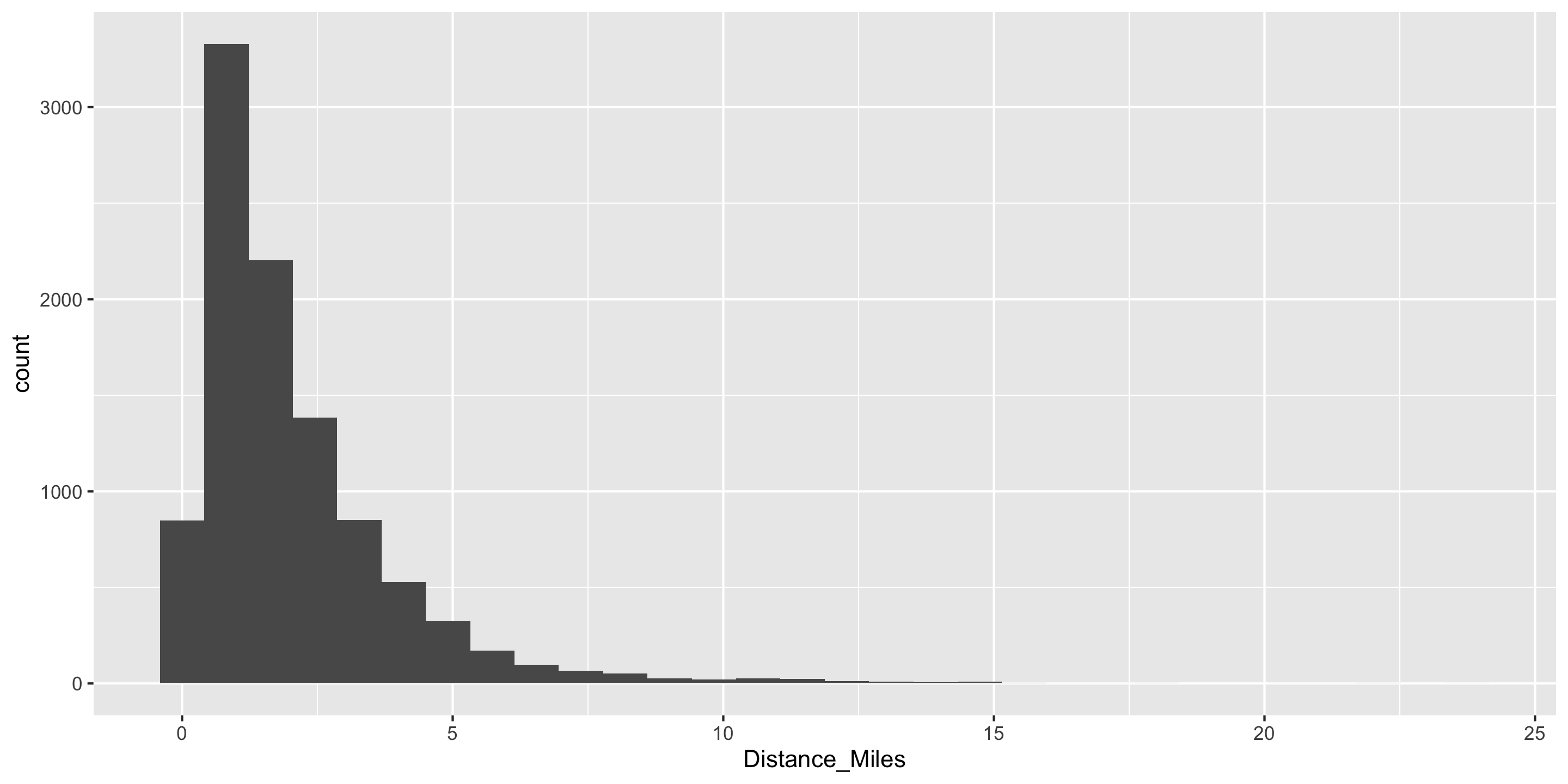
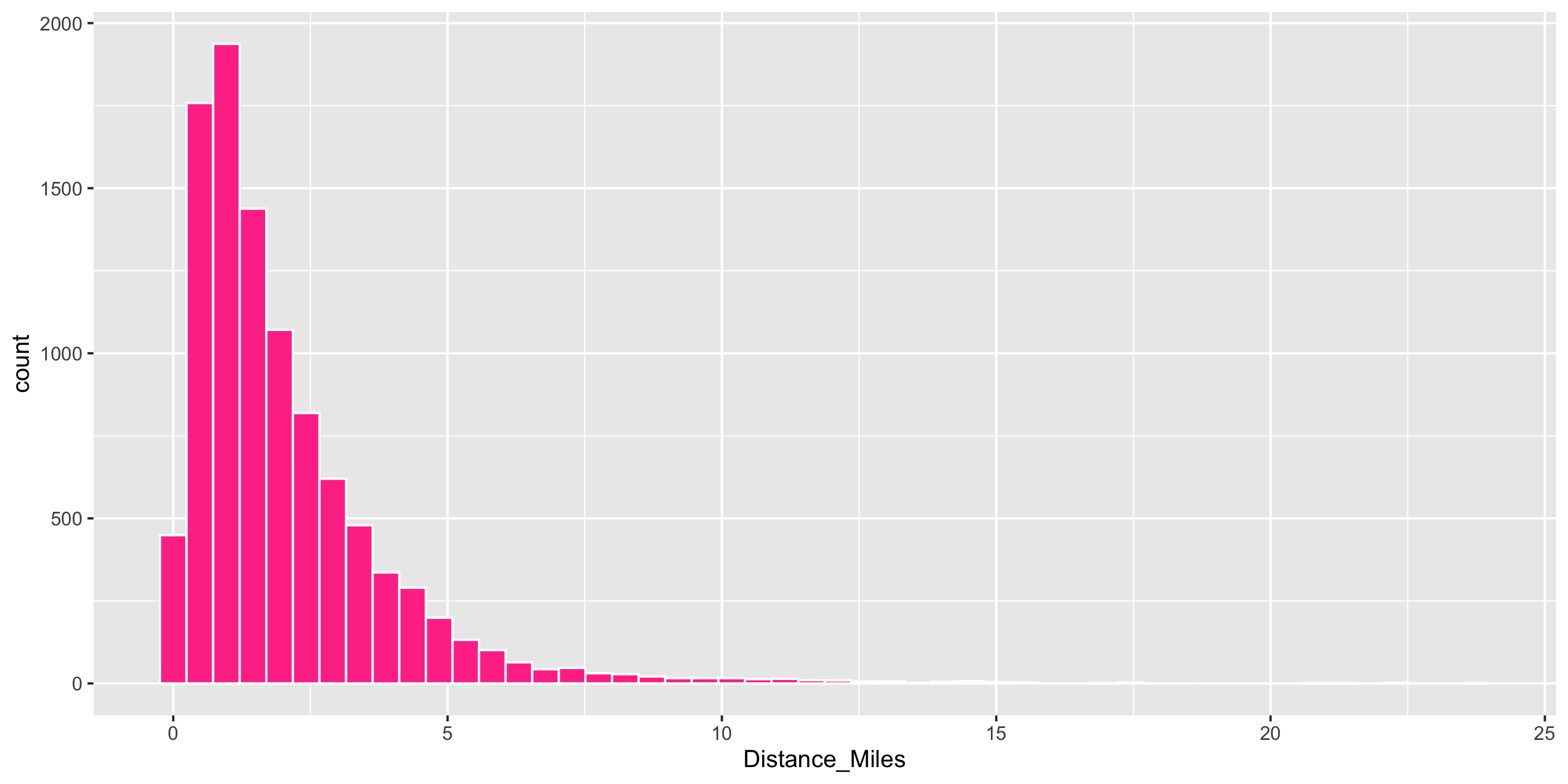
Histograms

• Binned counts of data.

• Great for assessing data distribution and shape.

• Question: are histograms used for quantitative or categorical variables?

• Answer: Quantitative.

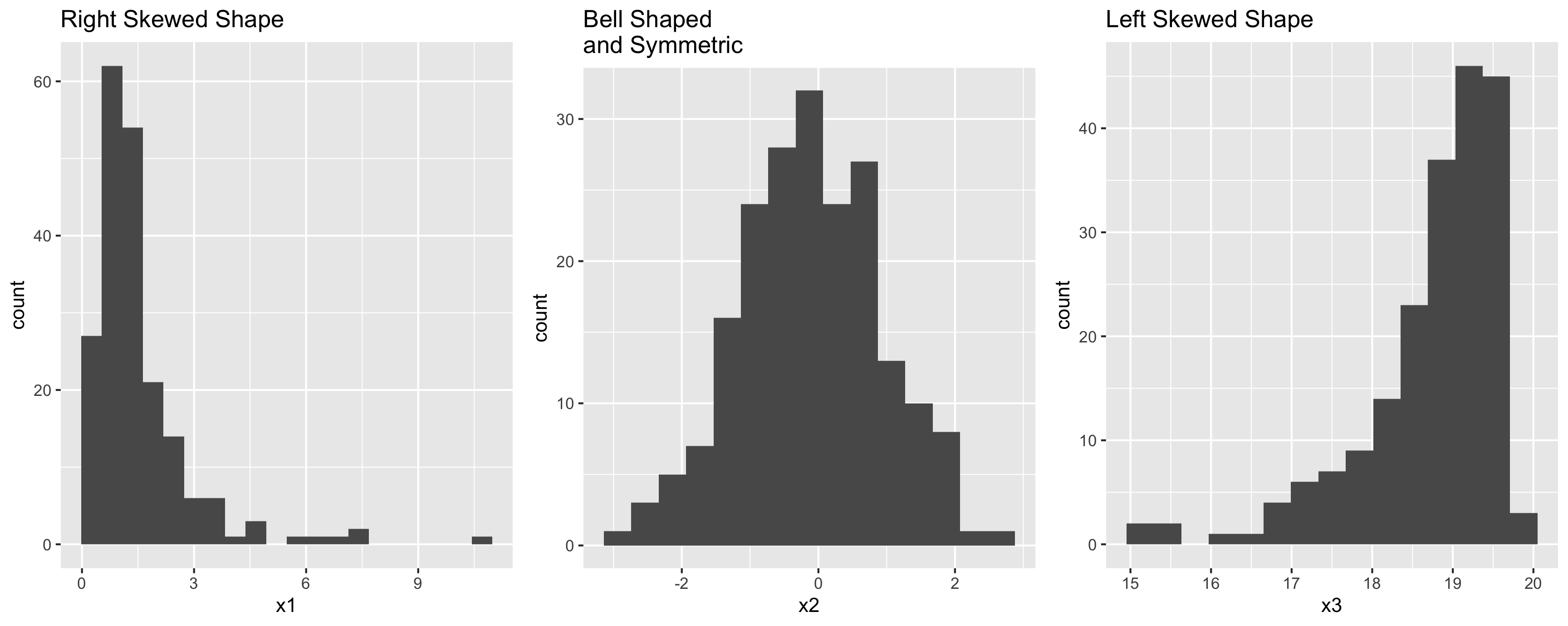
Data Shapes

Histograms

# Create histogram
ggplot(data = biketown, 
       mapping = aes(x = Distance_Miles)) +
  geom_histogram()

Histograms

# Create histogram
ggplot(data = biketown, 
       mapping = aes(x = Distance_Miles)) +
  geom_histogram(color = "white",
                 fill = "violetred1",
                 bins = 50)

• mapping to a variable goes in aes()
• setting to a specific, constant, value goes in the geom_---()
  
  
• Does the right tail of this distribution make sense?

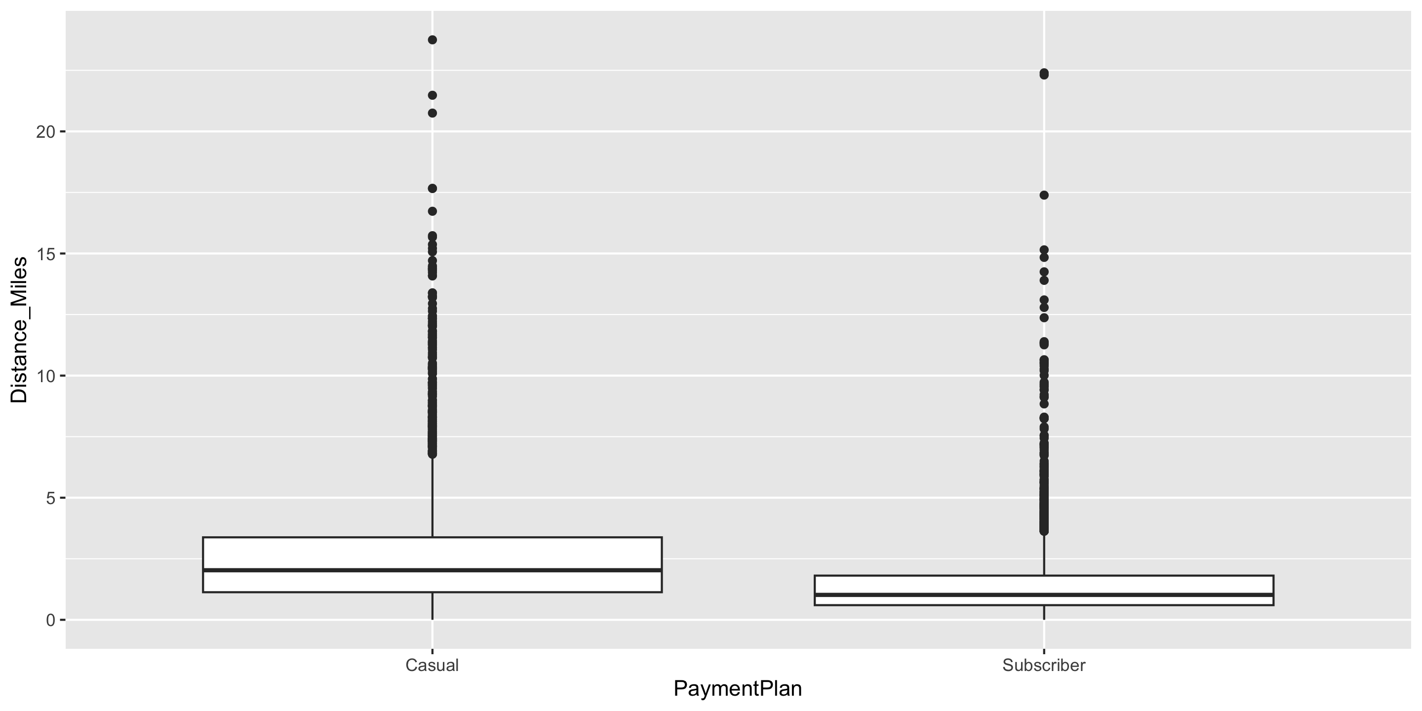
Boxplots

• Five number summary:
  • Minimum
  • First quartile (Q1)
  • Median
  • Third quartile (Q3)
  • Maximum
• Interquartile range (IQR) \(=\) Q3 \(-\) Q1
• Outliers: unusual points
  • Boxplot defines unusual as being beyond \(1.5*IQR\) from \(Q1\) or \(Q3\).
• Whiskers: reach out to the furthest point that is NOT an outlier

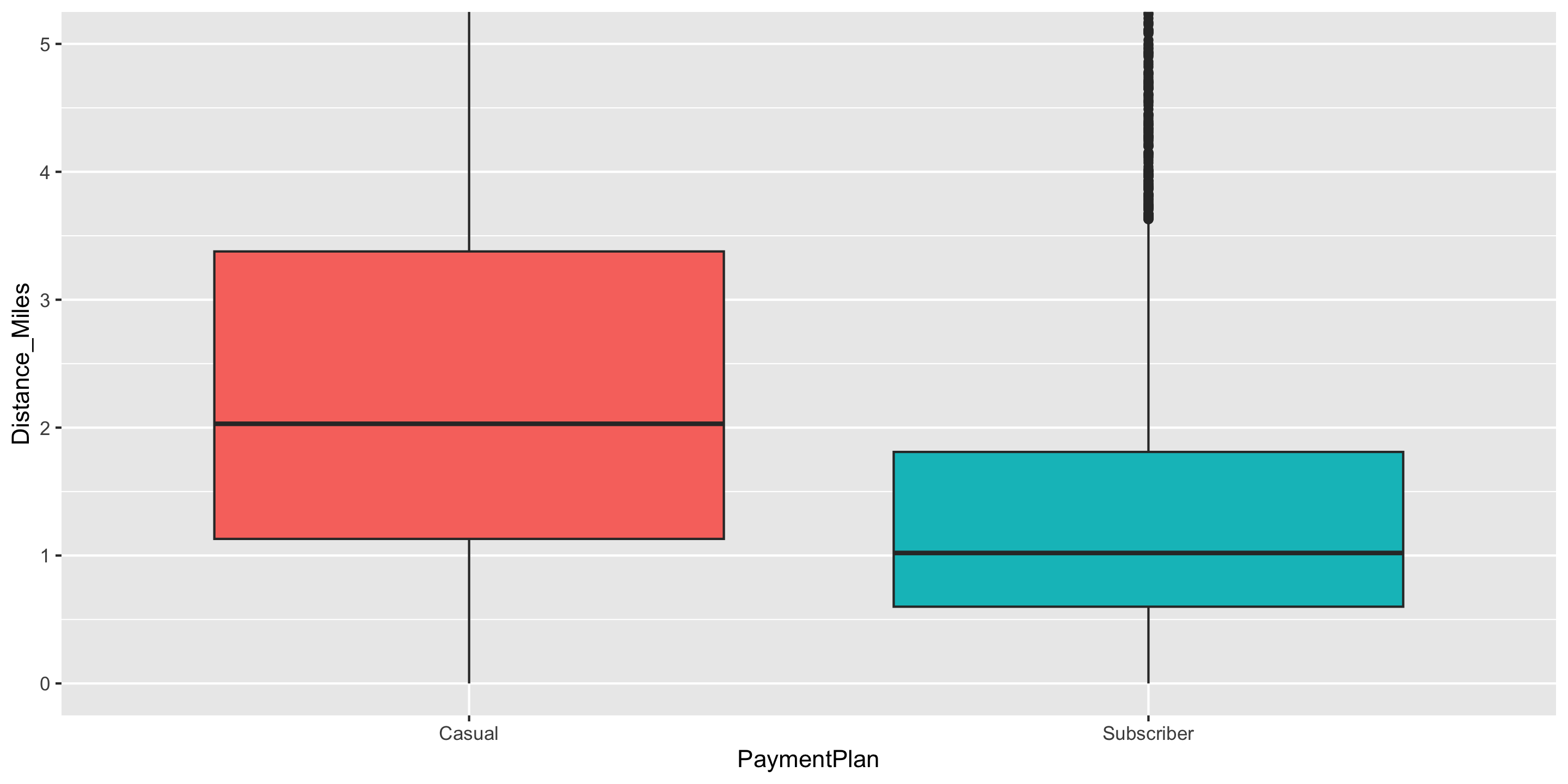
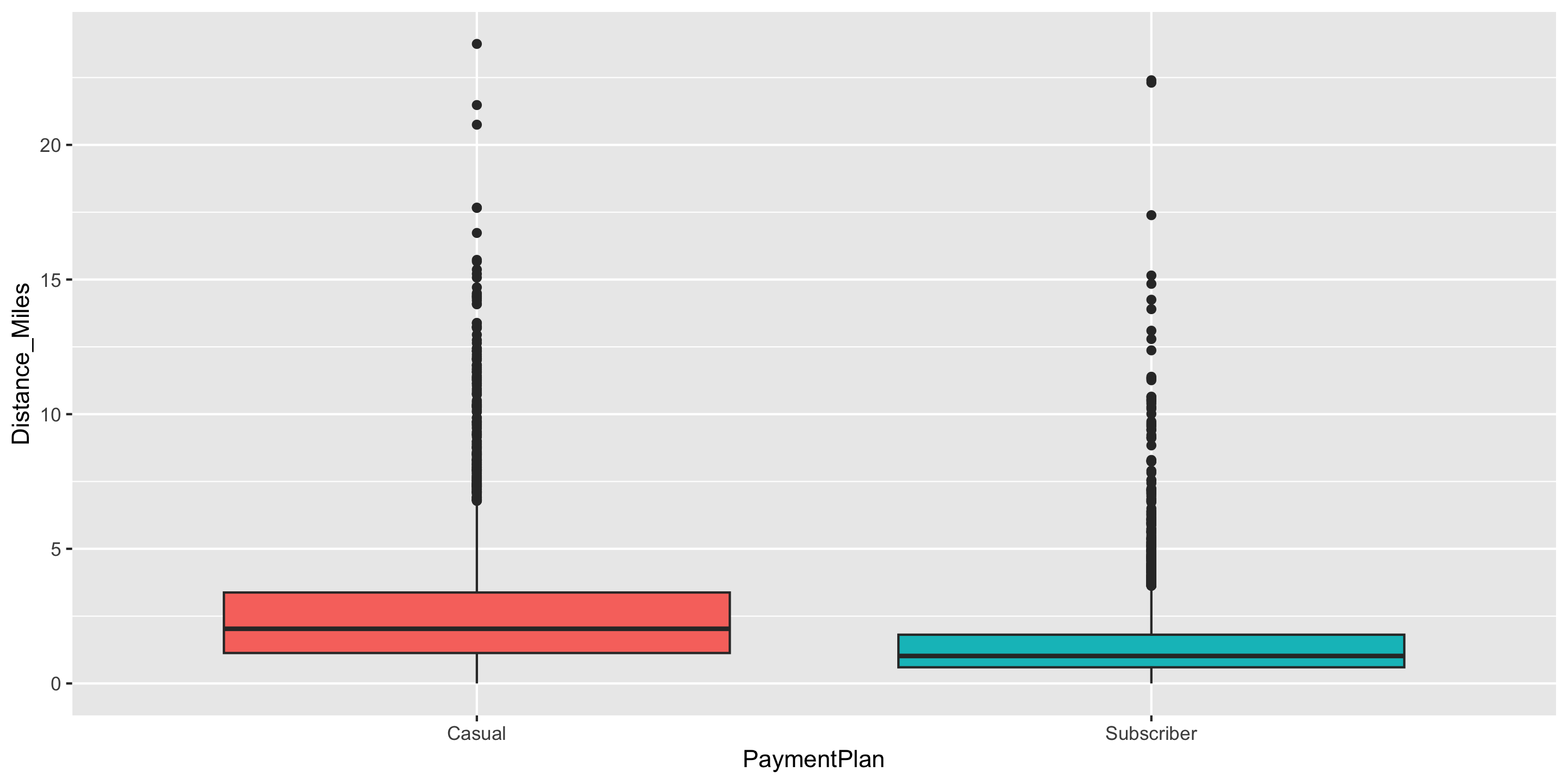
Boxplots

# Create boxplot
ggplot(data = biketown, 
       mapping = aes(x = PaymentPlan, 
                     y = Distance_Miles)) +
  geom_boxplot()

Boxplots

ggplot(data = biketown, 
       mapping = aes(x = PaymentPlan, 
                     y = Distance_Miles)) +
  geom_boxplot(fill = "springgreen3")

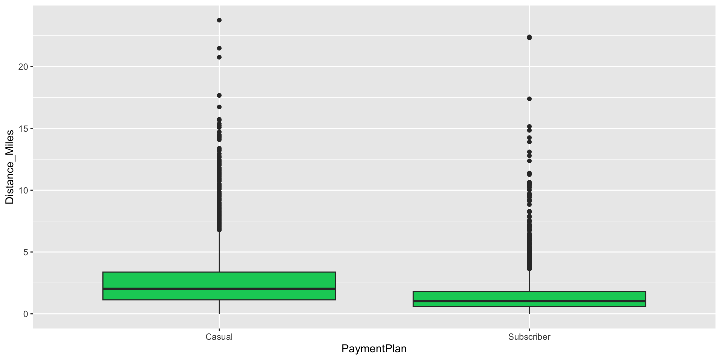
• Is this fill an aesthetic mapping?

Boxplots

ggplot(data = biketown, 
       mapping = aes(x = PaymentPlan, 
                     y = Distance_Miles,
                     fill = PaymentPlan)) +
  geom_boxplot()

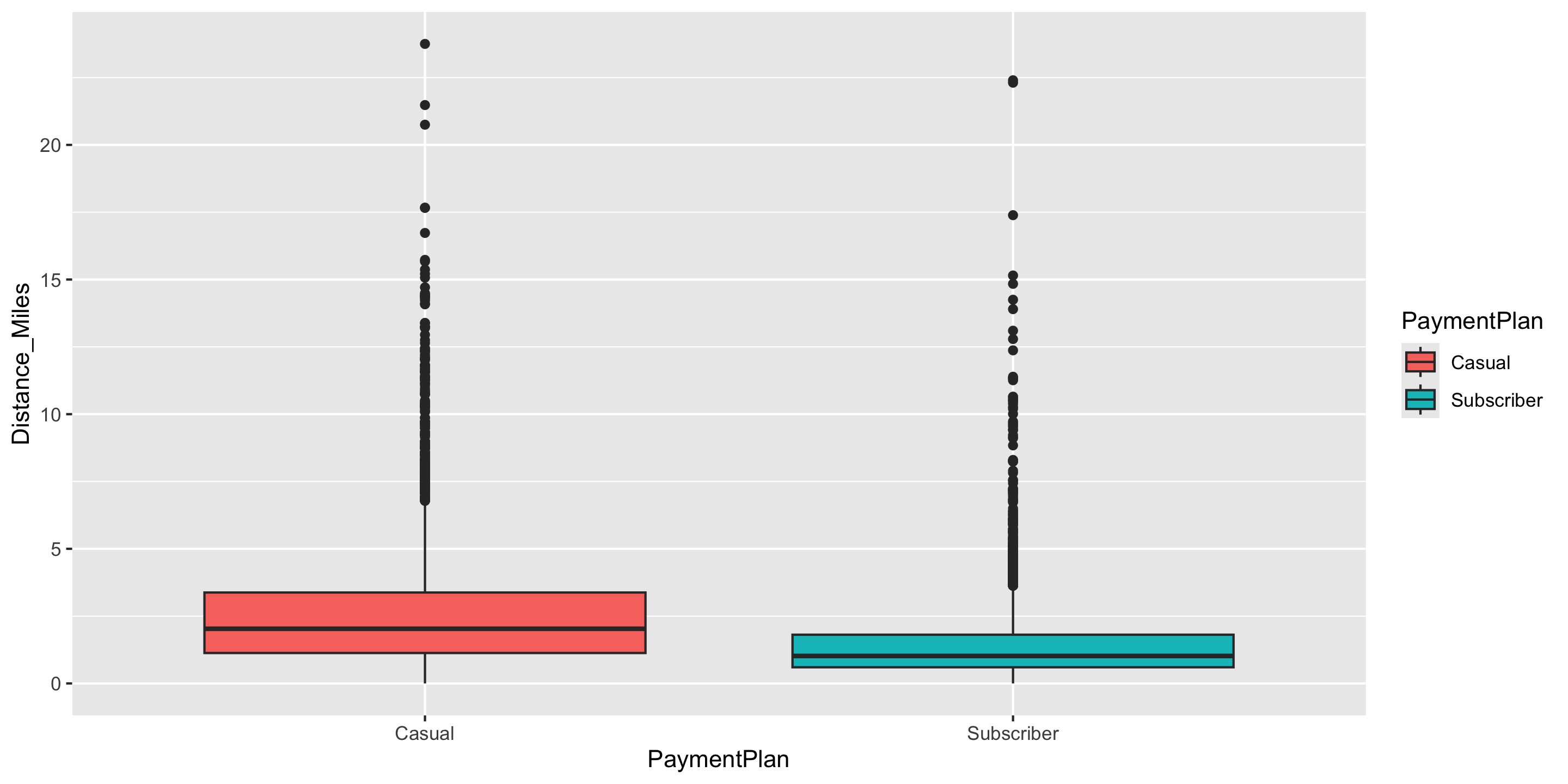
• Is this fill an aesthetic mapping?

• What variable is mapped to fill?

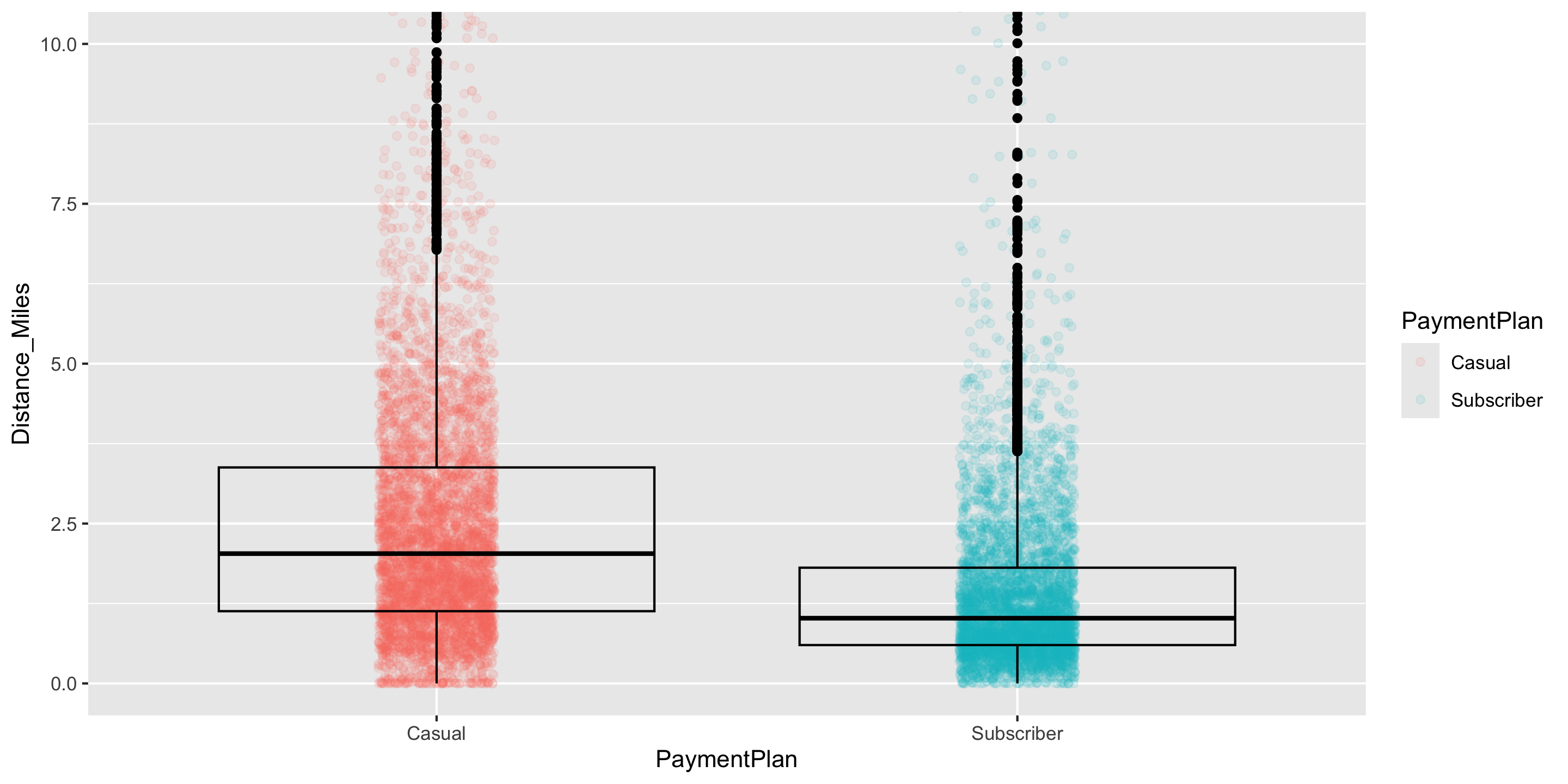
Boxplots

ggplot(data = biketown, 
       mapping = aes(x = PaymentPlan, 
                     y = Distance_Miles,
                     fill = PaymentPlan)) +
  geom_boxplot() +
  guides(fill = "none")

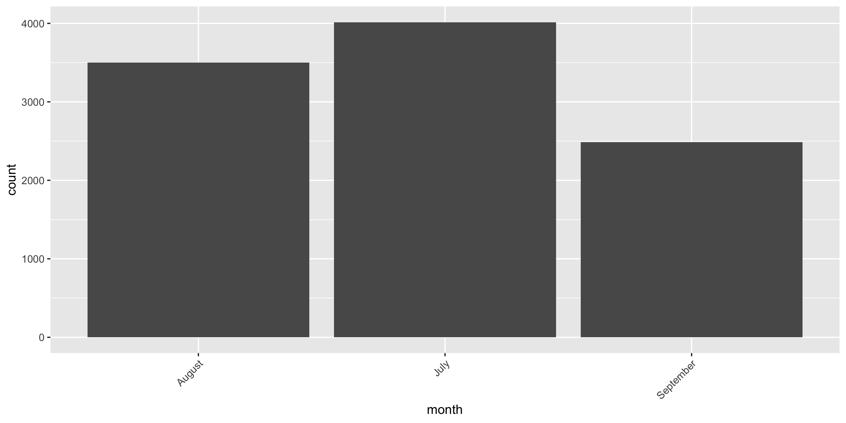
Barplots

ggplot(data = biketown, 
       mapping = aes(x = month)) +
  geom_bar()

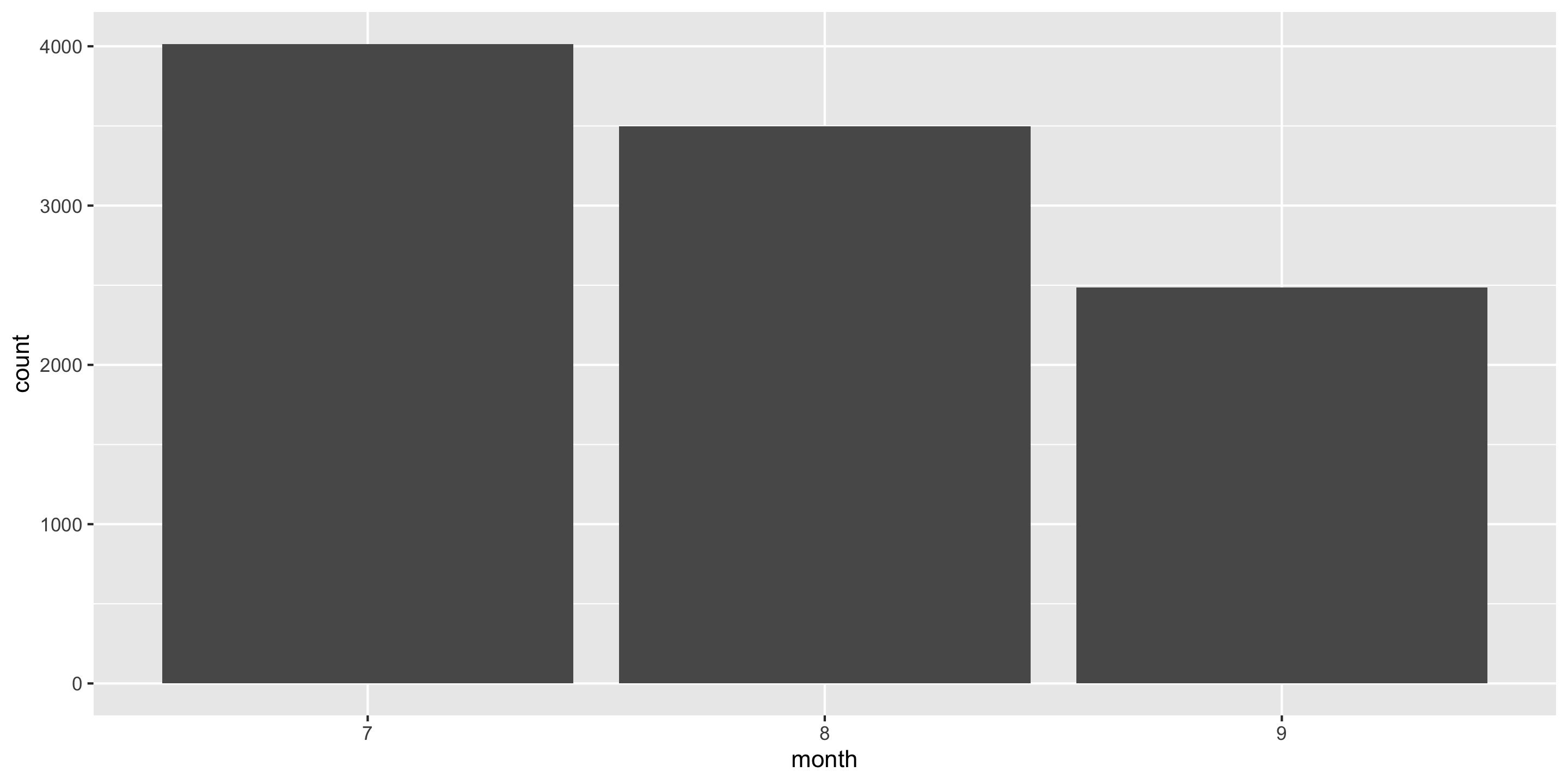
• Boxplots and histograms show the overall distribution of quantitative variables
• Barplots show the distribution of quantitative variables within distinct levels defined by a categorical variable

Barplots

ggplot(data = biketown, 
       mapping = aes(x = month,
                     fill = PaymentPlan)) +
  geom_bar()

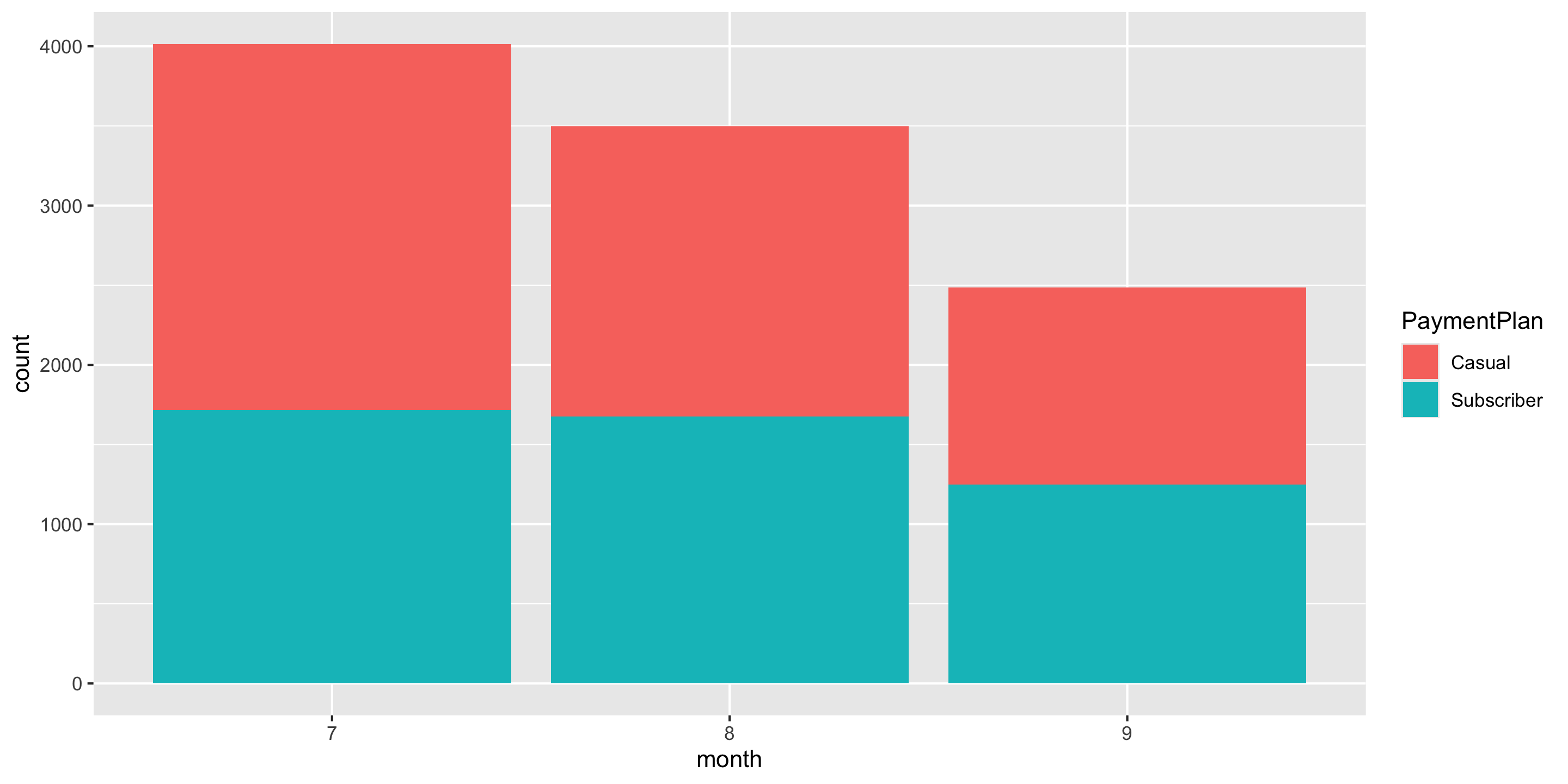
• Barplots can also show the joint distribution of two categorical variables via the color or fill aesthetic.
• Here, each bar is divided into separate counts with respect to the Payment Plan variable.

Barplots

ggplot(data = biketown, 
       mapping = aes(x = month,
                     fill = PaymentPlan)) +
  geom_bar(position = "fill")

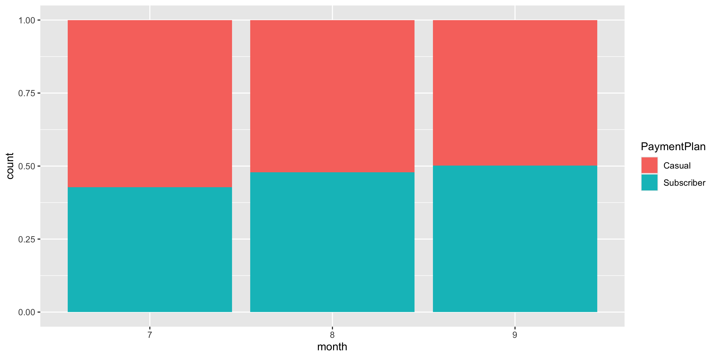
• Alternatively, we can consider the y-axis to represent proportion, making direct comparison easier.

New Data Context: pdxTrees

• The pdxTrees R package contains data on all the trees in the Portland Metro Area.
• Today, we’ll look at the Maple, Oak, Pine, Cedar, and Douglas-fir trees in a few parks near Reed.
• Let’s load the data

New Data Context: pdxTrees

• The pdxTrees R package contains data on all the trees in the Portland Metro Area.
• Today, we’ll look at the Maple, Oak, Pine, Cedar, and Douglas-fir trees in a few parks near Reed.
• Let’s load the data
• Don’t worry, we haven’t learned the below code yet.

library(pdxTrees)
near_Reed <- get_pdxTrees_parks(park = c("Woodstock Park", "Sellwood Riverfront Park", "Kenilworth Park"))
near_Reed <- near_Reed[near_Reed$Genus %in% c("Acer", "Quercus", "Pinus", "Thuja", "Pseudotsuga"), ]

Inspect the data

glimpse(near_Reed)

Rows: 323
Columns: 34
$ Longitude                  <dbl> -122.6304, -122.6301, -122.6301, -122.6299,…
$ Latitude                   <dbl> 45.49201, 45.49080, 45.49081, 45.49094, 45.…
$ UserID                     <chr> "7670", "7671", "7672", "7902", "7903", "79…
$ Genus                      <chr> "Quercus", "Pseudotsuga", "Pseudotsuga", "Q…
$ Family                     <chr> "Fagaceae", "Pinaceae", "Pinaceae", "Fagace…
$ DBH                        <dbl> 3.3, 43.1, 48.2, 2.4, 11.7, 33.5, 23.5, 37.…
$ Inventory_Date             <dttm> 2018-07-26, 2018-07-26, 2018-07-26, 2018-0…
$ Species                    <chr> "QURU", "PSME", "PSME", "QURU", "PSME", "PS…
$ Common_Name                <chr> "Northern Red Oak", "Douglas-Fir", "Douglas…
$ Condition                  <chr> "Fair", "Fair", "Fair", "Fair", "Good", "Fa…
$ Tree_Height                <dbl> 16, 148, 148, 16, 64, 118, 121, 105, 24, 12…
$ Crown_Width_NS             <dbl> 14, 61, 52, 9, 29, 32, 37, 43, 38, 44, 31, …
$ Crown_Width_EW             <dbl> 10, 43, 48, 14, 32, 50, 31, 44, 35, 36, 33,…
$ Crown_Base_Height          <dbl> 5, 6, 7, 2, 3, 60, 27, 10, 5, 19, 17, 6, 5,…
$ Collected_By               <chr> "Staff", "Staff", "Staff", "Staff", "Staff"…
$ Park                       <chr> "Kenilworth Park", "Kenilworth Park", "Keni…
$ Scientific_Name            <chr> "Quercus rubra", "Pseudotsuga menziesii", "…
$ Functional_Type            <chr> "BD", "CE", "CE", "BD", "CE", "CE", "CE", "…
$ Mature_Size                <fct> L, L, L, L, L, L, L, L, S, L, L, L, L, L, L…
$ Native                     <chr> "No", "Yes", "Yes", "No", "Yes", "Yes", "Ye…
$ Edible                     <chr> NA, NA, NA, NA, NA, NA, NA, NA, NA, NA, NA,…
$ Nuisance                   <chr> NA, NA, NA, NA, NA, NA, NA, NA, NA, NA, NA,…
$ Structural_Value           <dbl> 288.80, 12462.74, 14395.22, 143.21, 1348.26…
$ Carbon_Storage_lb          <dbl> 25.2, 4221.2, 5206.7, 11.6, 285.3, 2513.2, …
$ Carbon_Storage_value       <dbl> 1.63, 273.80, 337.73, 0.75, 18.51, 163.01, …
$ Carbon_Sequestration_lb    <dbl> 3.7, 43.5, 49.8, 2.4, 9.6, 32.4, 21.4, 37.4…
$ Carbon_Sequestration_value <dbl> 0.24, 2.82, 3.23, 0.15, 0.62, 2.10, 1.39, 2…
$ Stormwater_ft              <dbl> 5.2, 157.1, 145.2, 4.7, 56.8, 73.3, 68.1, 1…
$ Stormwater_value           <dbl> 0.35, 10.50, 9.71, 0.31, 3.80, 4.90, 4.55, …
$ Pollution_Removal_value    <dbl> 0.63, 19.08, 17.64, 0.57, 6.90, 8.90, 8.27,…
$ Pollution_Removal_oz       <dbl> 1.4, 42.3, 39.1, 1.3, 15.3, 19.7, 18.3, 30.…
$ Total_Annual_Services      <dbl> 1.21, 32.40, 30.58, 1.04, 11.31, 15.90, 14.…
$ Origin                     <chr> "North America - eastern Canada and eastern…
$ Species_Factoid            <chr> "Acorns take two years to mature and are an…

Inspect the data

head(near_Reed)

# A tibble: 6 × 34
  Longitude Latitude UserID Genus       Family   DBH Inventory_Date      Species
      <dbl>    <dbl> <chr>  <chr>       <chr>  <dbl> <dttm>              <chr>  
1     -123.     45.5 7670   Quercus     Fagac…   3.3 2018-07-26 00:00:00 QURU   
2     -123.     45.5 7671   Pseudotsuga Pinac…  43.1 2018-07-26 00:00:00 PSME   
3     -123.     45.5 7672   Pseudotsuga Pinac…  48.2 2018-07-26 00:00:00 PSME   
4     -123.     45.5 7902   Quercus     Fagac…   2.4 2018-07-26 00:00:00 QURU   
5     -123.     45.5 7903   Pseudotsuga Pinac…  11.7 2018-07-26 00:00:00 PSME   
6     -123.     45.5 7905   Pseudotsuga Pinac…  33.5 2018-07-26 00:00:00 PSME   
# ℹ 26 more variables: Common_Name <chr>, Condition <chr>, Tree_Height <dbl>,
#   Crown_Width_NS <dbl>, Crown_Width_EW <dbl>, Crown_Base_Height <dbl>,
#   Collected_By <chr>, Park <chr>, Scientific_Name <chr>,
#   Functional_Type <chr>, Mature_Size <fct>, Native <chr>, Edible <chr>,
#   Nuisance <chr>, Structural_Value <dbl>, Carbon_Storage_lb <dbl>,
#   Carbon_Storage_value <dbl>, Carbon_Sequestration_lb <dbl>,
#   Carbon_Sequestration_value <dbl>, Stormwater_ft <dbl>, …

What does a row represent here?

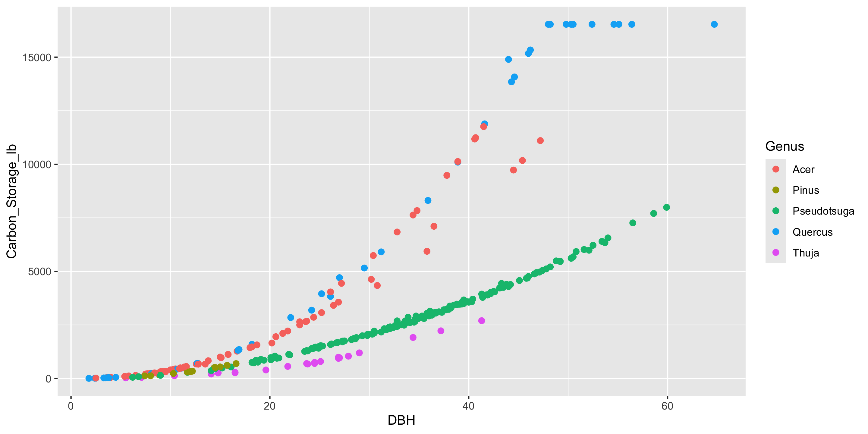
Scatterplots

• Explore relationships between numerical variables.
  • We will be especially interested in linear relationships.

ggplot(data = near_Reed,
       mapping = aes(x = DBH,
                     y = Carbon_Storage_lb)) +
  geom_point(size = 2)

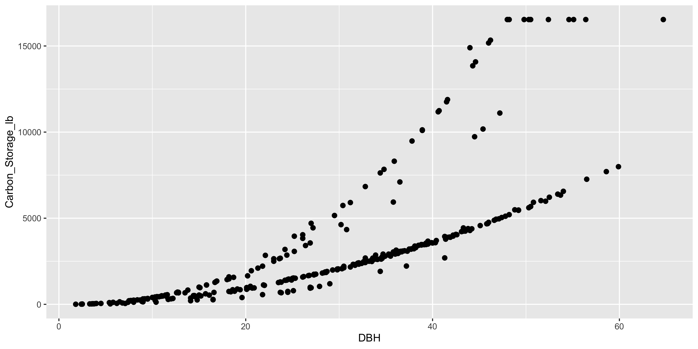
Is there something visually off with the points in this graph?

Scatterplots

ggplot(data = near_Reed,
       mapping = aes(x = DBH,
                     y = Carbon_Storage_lb)) +
  geom_point(size = 2, alpha = 0.25)

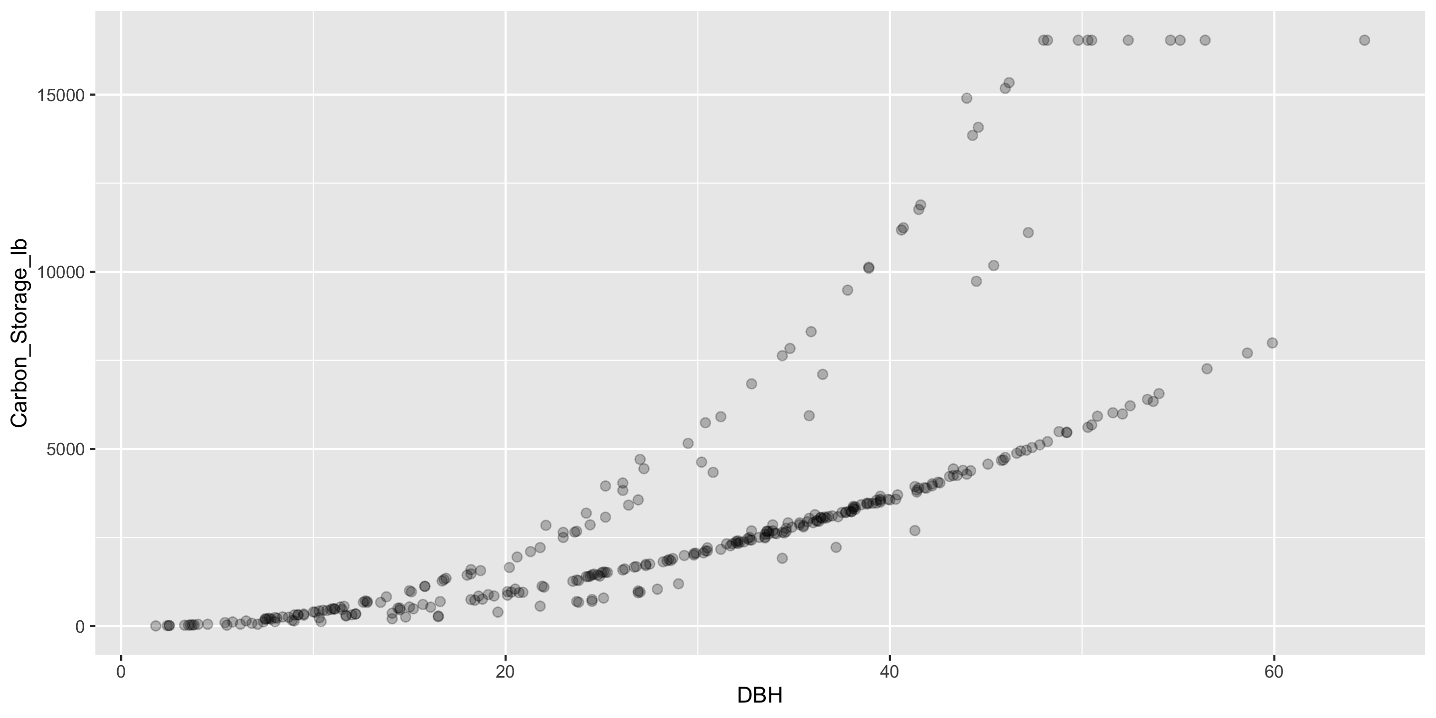
• Fix over-plotting (using alpha)
• What’s going on in this graph?

Scatterplots

ggplot(data = near_Reed,
       mapping = aes(x = DBH,
                     y = Carbon_Storage_lb)) +
  geom_point(size = 2, alpha = 0.25) +
  labs(x = "Diameter at Breast Height",
       y = "Carbon Storage (lbs)",
       caption = "Data Collected as part of the Urban Forestry Tree Inventory Project",
       title = "Tree Species Relationships Near Reed College")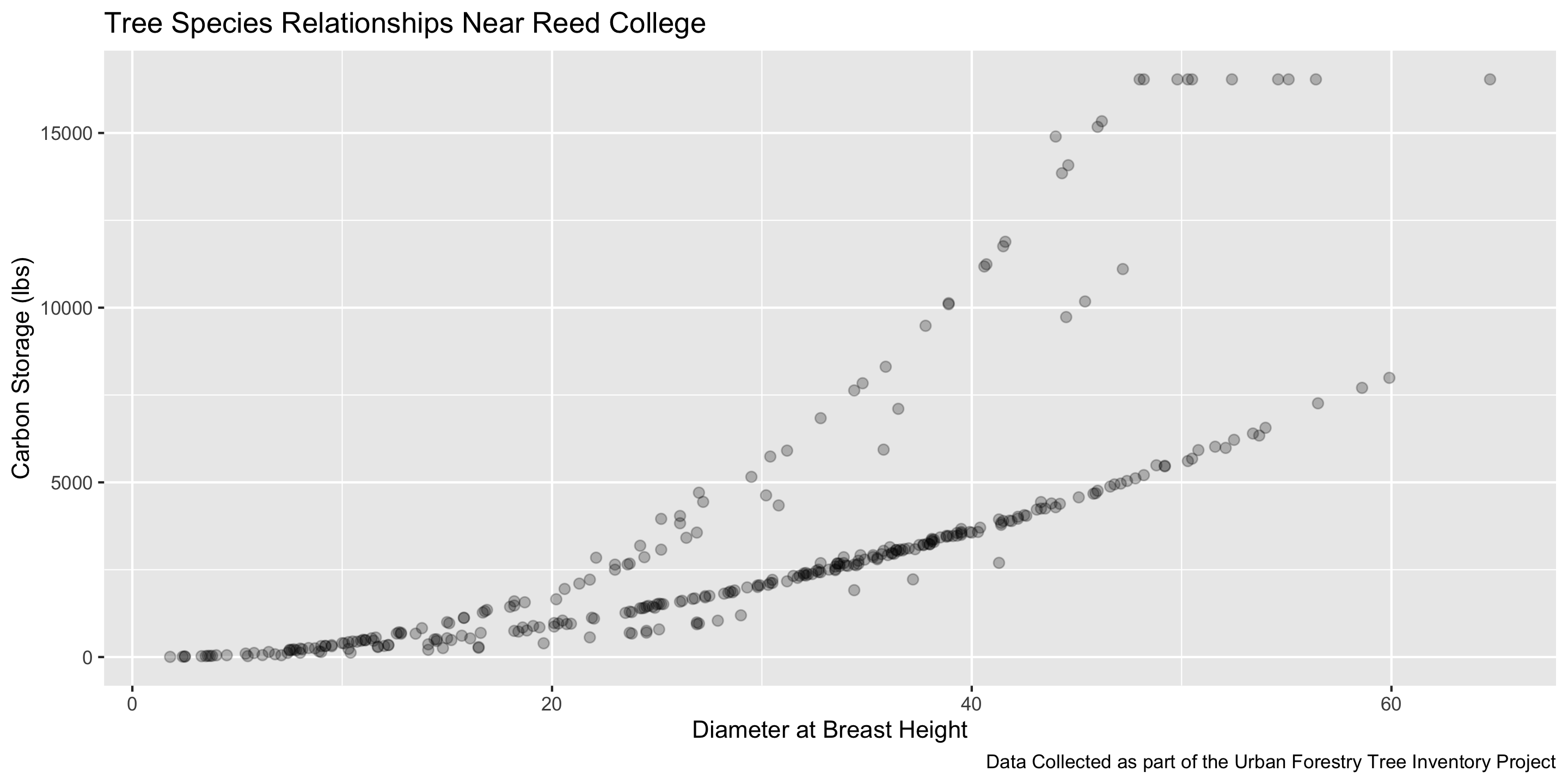

• Fix over-plotting (using alpha)
• What’s going on in this graph? (labels help add context)

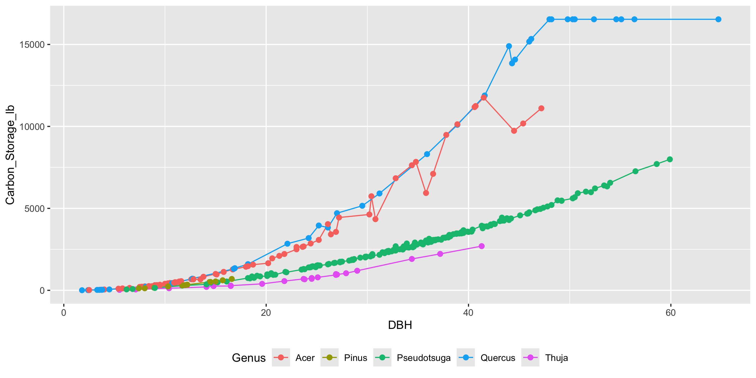
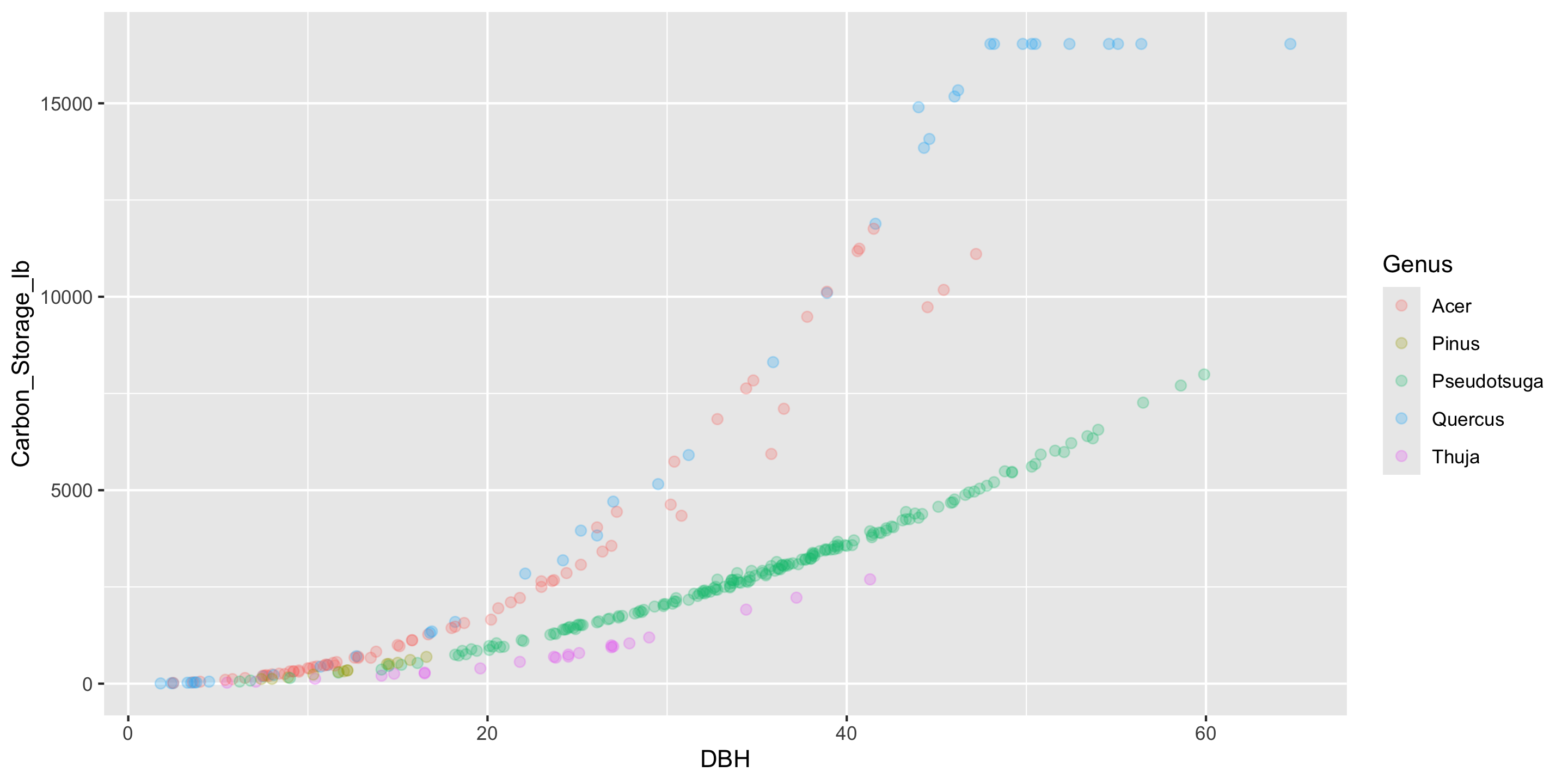
Scatterplots

ggplot(data = near_Reed,
       mapping = aes(x = DBH,
                     y = Carbon_Storage_lb,
                     color = Genus)) +
  geom_point(size = 2, alpha = 0.25)

Linegraphs

ggplot(data = near_Reed,
       mapping = aes(x = DBH,
                     y = Carbon_Storage_lb)) +
  geom_line(linewidth = 2)

Linegraphs

ggplot(data = near_Reed,
       mapping = aes(x = DBH,
                     y = Carbon_Storage_lb,
                     color = Genus)) +
  geom_line(linewidth = 2)

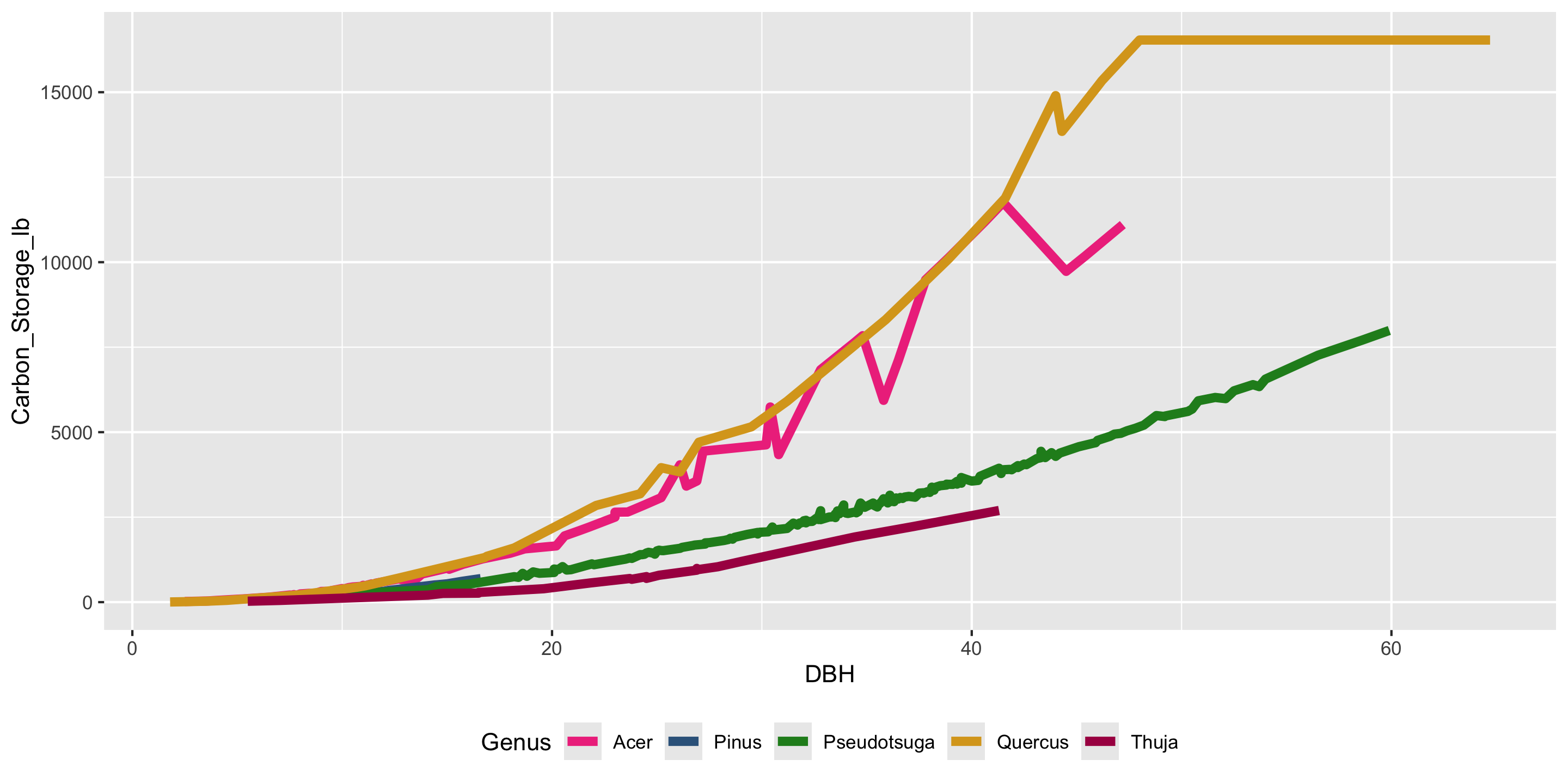
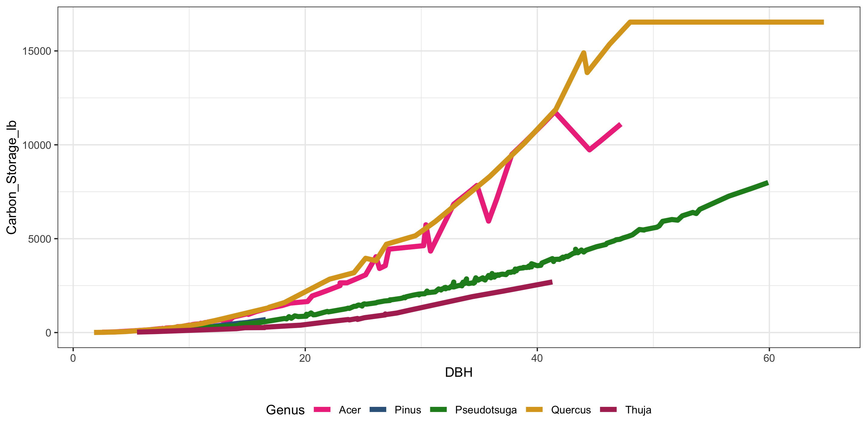
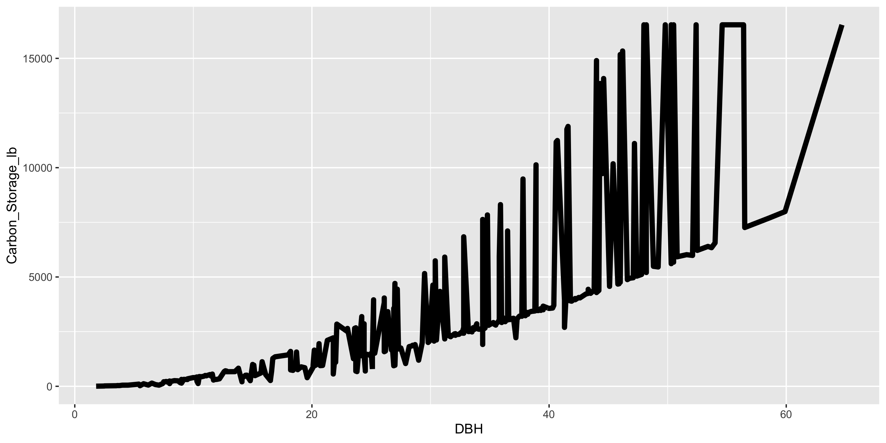
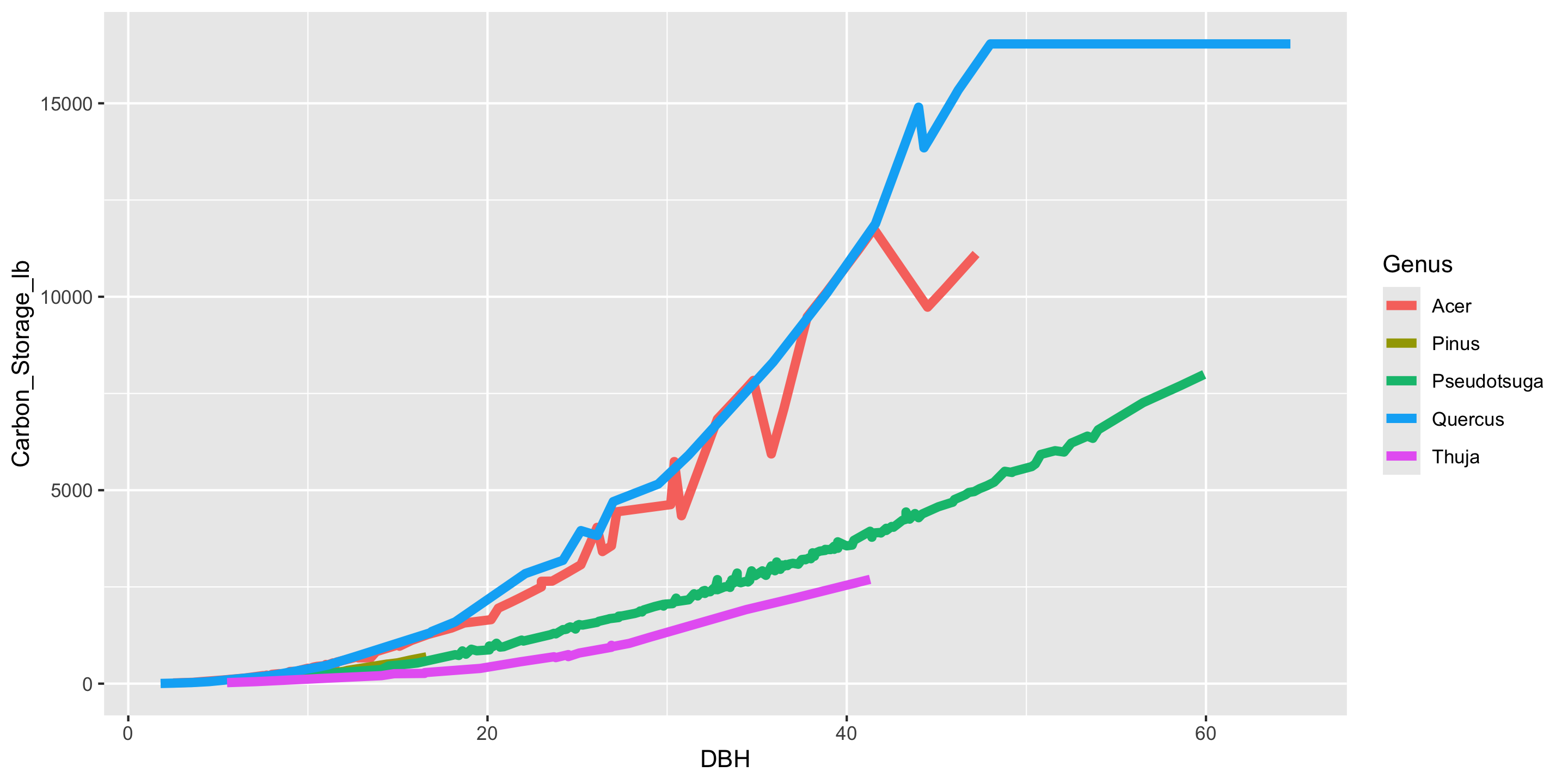
Linegraphs vs scatterplots

• Which do you prefer?
• Does it depend on context?

A speedy peek at advanced techniques!

If we run out of time, we’ll pick this back up during lab next Thursday.

Faceting

ggplot(data = near_Reed,
       mapping = aes(x = DBH,
                     y = Carbon_Storage_lb,
                     color = Genus)) +
  geom_line(linewidth = 2) +
  facet_wrap(~Genus) +
  guides(color = "none")

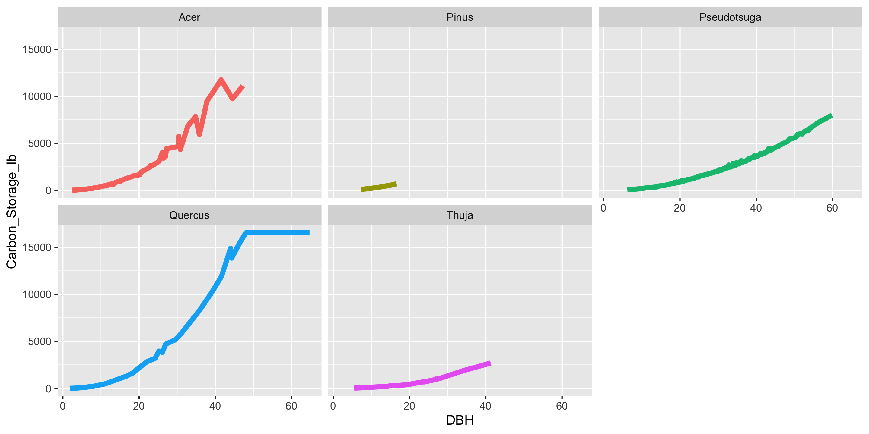
• Faceting is used to split one graphic into several smaller ones, based on the values of a categorical variable

Customizing your ggplot2 Plots

• There are so many ways you can customize the look of your ggplot2 plots

• Let’s look quickly at some common changes:

  • Fussing with labels
  • Zooming in
  • Using multiple geoms
  • Color!
  • Themes

Fussing with Labels: Rotate

biketown$month <- ifelse(biketown$month == 7, "July",
                         ifelse(biketown$month == 8, "August", "September"))
ggplot(data = biketown, 
       mapping = aes(x = month)) +
  geom_bar() +
    theme(axis.text.x =
          element_text(angle = 45,
                       vjust = 1,
                       hjust = 1))

Zooming In

ggplot(data = biketown, 
       mapping = aes(x = PaymentPlan, 
                     y = Distance_Miles,
                     fill = PaymentPlan)) +
  geom_boxplot() +
  guides(fill = "none")

Zooming In

ggplot(data = biketown, 
       mapping = aes(x = PaymentPlan, 
                     y = Distance_Miles,
                     fill = PaymentPlan)) +
  geom_boxplot() +
  guides(fill = "none") +
  coord_cartesian(ylim = c(0, 5))

Multiple geoms

ggplot(data = biketown, 
       mapping = aes(x = PaymentPlan, 
                     y = Distance_Miles,
                     color = PaymentPlan)) +
  guides(fill = "none") +
  coord_cartesian(ylim = c(0, 10)) +
  geom_jitter(width = 0.1,
              height = 0, 
              alpha = 0.1) +
    geom_boxplot(fill = NA, color = "black")

Multiple geoms

ggplot(data = near_Reed,
       mapping = aes(x = DBH,
                     y = Carbon_Storage_lb,
                     color = Genus)) +
  geom_line() +
  theme(legend.position = "bottom") +
  geom_point(size = 2)

Change the Color

colors()

  [1] "white"                "aliceblue"            "antiquewhite"        
  [4] "antiquewhite1"        "antiquewhite2"        "antiquewhite3"       
  [7] "antiquewhite4"        "aquamarine"           "aquamarine1"         
 [10] "aquamarine2"          "aquamarine3"          "aquamarine4"         
 [13] "azure"                "azure1"               "azure2"              
 [16] "azure3"               "azure4"               "beige"               
 [19] "bisque"               "bisque1"              "bisque2"             
 [22] "bisque3"              "bisque4"              "black"               
 [25] "blanchedalmond"       "blue"                 "blue1"               
 [28] "blue2"                "blue3"                "blue4"               
 [31] "blueviolet"           "brown"                "brown1"              
 [34] "brown2"               "brown3"               "brown4"              
 [37] "burlywood"            "burlywood1"           "burlywood2"          
 [40] "burlywood3"           "burlywood4"           "cadetblue"           
 [43] "cadetblue1"           "cadetblue2"           "cadetblue3"          
 [46] "cadetblue4"           "chartreuse"           "chartreuse1"         
 [49] "chartreuse2"          "chartreuse3"          "chartreuse4"         
 [52] "chocolate"            "chocolate1"           "chocolate2"          
 [55] "chocolate3"           "chocolate4"           "coral"               
 [58] "coral1"               "coral2"               "coral3"              
 [61] "coral4"               "cornflowerblue"       "cornsilk"            
 [64] "cornsilk1"            "cornsilk2"            "cornsilk3"           
 [67] "cornsilk4"            "cyan"                 "cyan1"               
 [70] "cyan2"                "cyan3"                "cyan4"               
 [73] "darkblue"             "darkcyan"             "darkgoldenrod"       
 [76] "darkgoldenrod1"       "darkgoldenrod2"       "darkgoldenrod3"      
 [79] "darkgoldenrod4"       "darkgray"             "darkgreen"           
 [82] "darkgrey"             "darkkhaki"            "darkmagenta"         
 [85] "darkolivegreen"       "darkolivegreen1"      "darkolivegreen2"     
 [88] "darkolivegreen3"      "darkolivegreen4"      "darkorange"          
 [91] "darkorange1"          "darkorange2"          "darkorange3"         
 [94] "darkorange4"          "darkorchid"           "darkorchid1"         
 [97] "darkorchid2"          "darkorchid3"          "darkorchid4"         
[100] "darkred"              "darksalmon"           "darkseagreen"        
[103] "darkseagreen1"        "darkseagreen2"        "darkseagreen3"       
[106] "darkseagreen4"        "darkslateblue"        "darkslategray"       
[109] "darkslategray1"       "darkslategray2"       "darkslategray3"      
[112] "darkslategray4"       "darkslategrey"        "darkturquoise"       
[115] "darkviolet"           "deeppink"             "deeppink1"           
[118] "deeppink2"            "deeppink3"            "deeppink4"           
[121] "deepskyblue"          "deepskyblue1"         "deepskyblue2"        
[124] "deepskyblue3"         "deepskyblue4"         "dimgray"             
[127] "dimgrey"              "dodgerblue"           "dodgerblue1"         
[130] "dodgerblue2"          "dodgerblue3"          "dodgerblue4"         
[133] "firebrick"            "firebrick1"           "firebrick2"          
[136] "firebrick3"           "firebrick4"           "floralwhite"         
[139] "forestgreen"          "gainsboro"            "ghostwhite"          
[142] "gold"                 "gold1"                "gold2"               
[145] "gold3"                "gold4"                "goldenrod"           
[148] "goldenrod1"           "goldenrod2"           "goldenrod3"          
[151] "goldenrod4"           "gray"                 "gray0"               
[154] "gray1"                "gray2"                "gray3"               
[157] "gray4"                "gray5"                "gray6"               
[160] "gray7"                "gray8"                "gray9"               
[163] "gray10"               "gray11"               "gray12"              
[166] "gray13"               "gray14"               "gray15"              
[169] "gray16"               "gray17"               "gray18"              
[172] "gray19"               "gray20"               "gray21"              
[175] "gray22"               "gray23"               "gray24"              
[178] "gray25"               "gray26"               "gray27"              
[181] "gray28"               "gray29"               "gray30"              
[184] "gray31"               "gray32"               "gray33"              
[187] "gray34"               "gray35"               "gray36"              
[190] "gray37"               "gray38"               "gray39"              
[193] "gray40"               "gray41"               "gray42"              
[196] "gray43"               "gray44"               "gray45"              
[199] "gray46"               "gray47"               "gray48"              
[202] "gray49"               "gray50"               "gray51"              
[205] "gray52"               "gray53"               "gray54"              
[208] "gray55"               "gray56"               "gray57"              
[211] "gray58"               "gray59"               "gray60"              
[214] "gray61"               "gray62"               "gray63"              
[217] "gray64"               "gray65"               "gray66"              
[220] "gray67"               "gray68"               "gray69"              
[223] "gray70"               "gray71"               "gray72"              
[226] "gray73"               "gray74"               "gray75"              
[229] "gray76"               "gray77"               "gray78"              
[232] "gray79"               "gray80"               "gray81"              
[235] "gray82"               "gray83"               "gray84"              
[238] "gray85"               "gray86"               "gray87"              
[241] "gray88"               "gray89"               "gray90"              
[244] "gray91"               "gray92"               "gray93"              
[247] "gray94"               "gray95"               "gray96"              
[250] "gray97"               "gray98"               "gray99"              
[253] "gray100"              "green"                "green1"              
[256] "green2"               "green3"               "green4"              
[259] "greenyellow"          "grey"                 "grey0"               
[262] "grey1"                "grey2"                "grey3"               
[265] "grey4"                "grey5"                "grey6"               
[268] "grey7"                "grey8"                "grey9"               
[271] "grey10"               "grey11"               "grey12"              
[274] "grey13"               "grey14"               "grey15"              
[277] "grey16"               "grey17"               "grey18"              
[280] "grey19"               "grey20"               "grey21"              
[283] "grey22"               "grey23"               "grey24"              
[286] "grey25"               "grey26"               "grey27"              
[289] "grey28"               "grey29"               "grey30"              
[292] "grey31"               "grey32"               "grey33"              
[295] "grey34"               "grey35"               "grey36"              
[298] "grey37"               "grey38"               "grey39"              
[301] "grey40"               "grey41"               "grey42"              
[304] "grey43"               "grey44"               "grey45"              
[307] "grey46"               "grey47"               "grey48"              
[310] "grey49"               "grey50"               "grey51"              
[313] "grey52"               "grey53"               "grey54"              
[316] "grey55"               "grey56"               "grey57"              
[319] "grey58"               "grey59"               "grey60"              
[322] "grey61"               "grey62"               "grey63"              
[325] "grey64"               "grey65"               "grey66"              
[328] "grey67"               "grey68"               "grey69"              
[331] "grey70"               "grey71"               "grey72"              
[334] "grey73"               "grey74"               "grey75"              
[337] "grey76"               "grey77"               "grey78"              
[340] "grey79"               "grey80"               "grey81"              
[343] "grey82"               "grey83"               "grey84"              
[346] "grey85"               "grey86"               "grey87"              
[349] "grey88"               "grey89"               "grey90"              
[352] "grey91"               "grey92"               "grey93"              
[355] "grey94"               "grey95"               "grey96"              
[358] "grey97"               "grey98"               "grey99"              
[361] "grey100"              "honeydew"             "honeydew1"           
[364] "honeydew2"            "honeydew3"            "honeydew4"           
[367] "hotpink"              "hotpink1"             "hotpink2"            
[370] "hotpink3"             "hotpink4"             "indianred"           
[373] "indianred1"           "indianred2"           "indianred3"          
[376] "indianred4"           "ivory"                "ivory1"              
[379] "ivory2"               "ivory3"               "ivory4"              
[382] "khaki"                "khaki1"               "khaki2"              
[385] "khaki3"               "khaki4"               "lavender"            
[388] "lavenderblush"        "lavenderblush1"       "lavenderblush2"      
[391] "lavenderblush3"       "lavenderblush4"       "lawngreen"           
[394] "lemonchiffon"         "lemonchiffon1"        "lemonchiffon2"       
[397] "lemonchiffon3"        "lemonchiffon4"        "lightblue"           
[400] "lightblue1"           "lightblue2"           "lightblue3"          
[403] "lightblue4"           "lightcoral"           "lightcyan"           
[406] "lightcyan1"           "lightcyan2"           "lightcyan3"          
[409] "lightcyan4"           "lightgoldenrod"       "lightgoldenrod1"     
[412] "lightgoldenrod2"      "lightgoldenrod3"      "lightgoldenrod4"     
[415] "lightgoldenrodyellow" "lightgray"            "lightgreen"          
[418] "lightgrey"            "lightpink"            "lightpink1"          
[421] "lightpink2"           "lightpink3"           "lightpink4"          
[424] "lightsalmon"          "lightsalmon1"         "lightsalmon2"        
[427] "lightsalmon3"         "lightsalmon4"         "lightseagreen"       
[430] "lightskyblue"         "lightskyblue1"        "lightskyblue2"       
[433] "lightskyblue3"        "lightskyblue4"        "lightslateblue"      
[436] "lightslategray"       "lightslategrey"       "lightsteelblue"      
[439] "lightsteelblue1"      "lightsteelblue2"      "lightsteelblue3"     
[442] "lightsteelblue4"      "lightyellow"          "lightyellow1"        
[445] "lightyellow2"         "lightyellow3"         "lightyellow4"        
[448] "limegreen"            "linen"                "magenta"             
[451] "magenta1"             "magenta2"             "magenta3"            
[454] "magenta4"             "maroon"               "maroon1"             
[457] "maroon2"              "maroon3"              "maroon4"             
[460] "mediumaquamarine"     "mediumblue"           "mediumorchid"        
[463] "mediumorchid1"        "mediumorchid2"        "mediumorchid3"       
[466] "mediumorchid4"        "mediumpurple"         "mediumpurple1"       
[469] "mediumpurple2"        "mediumpurple3"        "mediumpurple4"       
[472] "mediumseagreen"       "mediumslateblue"      "mediumspringgreen"   
[475] "mediumturquoise"      "mediumvioletred"      "midnightblue"        
[478] "mintcream"            "mistyrose"            "mistyrose1"          
[481] "mistyrose2"           "mistyrose3"           "mistyrose4"          
[484] "moccasin"             "navajowhite"          "navajowhite1"        
[487] "navajowhite2"         "navajowhite3"         "navajowhite4"        
[490] "navy"                 "navyblue"             "oldlace"             
[493] "olivedrab"            "olivedrab1"           "olivedrab2"          
[496] "olivedrab3"           "olivedrab4"           "orange"              
[499] "orange1"              "orange2"              "orange3"             
[502] "orange4"              "orangered"            "orangered1"          
[505] "orangered2"           "orangered3"           "orangered4"          
[508] "orchid"               "orchid1"              "orchid2"             
[511] "orchid3"              "orchid4"              "palegoldenrod"       
[514] "palegreen"            "palegreen1"           "palegreen2"          
[517] "palegreen3"           "palegreen4"           "paleturquoise"       
[520] "paleturquoise1"       "paleturquoise2"       "paleturquoise3"      
[523] "paleturquoise4"       "palevioletred"        "palevioletred1"      
[526] "palevioletred2"       "palevioletred3"       "palevioletred4"      
[529] "papayawhip"           "peachpuff"            "peachpuff1"          
[532] "peachpuff2"           "peachpuff3"           "peachpuff4"          
[535] "peru"                 "pink"                 "pink1"               
[538] "pink2"                "pink3"                "pink4"               
[541] "plum"                 "plum1"                "plum2"               
[544] "plum3"                "plum4"                "powderblue"          
[547] "purple"               "purple1"              "purple2"             
[550] "purple3"              "purple4"              "red"                 
[553] "red1"                 "red2"                 "red3"                
[556] "red4"                 "rosybrown"            "rosybrown1"          
[559] "rosybrown2"           "rosybrown3"           "rosybrown4"          
[562] "royalblue"            "royalblue1"           "royalblue2"          
[565] "royalblue3"           "royalblue4"           "saddlebrown"         
[568] "salmon"               "salmon1"              "salmon2"             
[571] "salmon3"              "salmon4"              "sandybrown"          
[574] "seagreen"             "seagreen1"            "seagreen2"           
[577] "seagreen3"            "seagreen4"            "seashell"            
[580] "seashell1"            "seashell2"            "seashell3"           
[583] "seashell4"            "sienna"               "sienna1"             
[586] "sienna2"              "sienna3"              "sienna4"             
[589] "skyblue"              "skyblue1"             "skyblue2"            
[592] "skyblue3"             "skyblue4"             "slateblue"           
[595] "slateblue1"           "slateblue2"           "slateblue3"          
[598] "slateblue4"           "slategray"            "slategray1"          
[601] "slategray2"           "slategray3"           "slategray4"          
[604] "slategrey"            "snow"                 "snow1"               
[607] "snow2"                "snow3"                "snow4"               
[610] "springgreen"          "springgreen1"         "springgreen2"        
[613] "springgreen3"         "springgreen4"         "steelblue"           
[616] "steelblue1"           "steelblue2"           "steelblue3"          
[619] "steelblue4"           "tan"                  "tan1"                
[622] "tan2"                 "tan3"                 "tan4"                
[625] "thistle"              "thistle1"             "thistle2"            
[628] "thistle3"             "thistle4"             "tomato"              
[631] "tomato1"              "tomato2"              "tomato3"             
[634] "tomato4"              "turquoise"            "turquoise1"          
[637] "turquoise2"           "turquoise3"           "turquoise4"          
[640] "violet"               "violetred"            "violetred1"          
[643] "violetred2"           "violetred3"           "violetred4"          
[646] "wheat"                "wheat1"               "wheat2"              
[649] "wheat3"               "wheat4"               "whitesmoke"          
[652] "yellow"               "yellow1"              "yellow2"             
[655] "yellow3"              "yellow4"              "yellowgreen"         

You can also use hex color codes to fully customize colors.

Change the Color

ggplot(data = near_Reed,
       mapping = aes(x = DBH,
                     y = Carbon_Storage_lb,
                     color = Genus)) +
  geom_line(size = 2) +
  theme(legend.position = "bottom") +
  scale_color_manual(values = c("violetred2",
                                "steelblue4",
                                "forestgreen",
                                "goldenrod",
                                "#aa0951"))

Use a Different Theme

ggplot(data = near_Reed,
       mapping = aes(x = DBH,
                     y = Carbon_Storage_lb,
                     color = Genus)) +
  geom_line(size = 2) +
  scale_color_manual(values = c("violetred2",
                                "steelblue4",
                                "forestgreen",
                                "goldenrod",
                                "maroon")) +
  theme_bw() +
  theme(legend.position = "bottom") 

Recap: ggplot2

library(tidyverse)
ggplot(data = ---, mapping = aes(---)) +
  geom_---(---) 

• This is the major concept to remember
• We covered a lot of ground - it takes lots of practice to become fluent in the details!

Next time:

• Data wrangling!